CS70: Jean Walrand: Lecture 25. Markov Chains: Distributions 1. - PowerPoint PPT Presentation
CS70: Jean Walrand: Lecture 25. Markov Chains: Distributions 1. Review 2. Distribution 3. Irreducibility 4. Convergence Review Markov Chain: Finite set X ; 0 ; P = { P ( i , j ) , i , j X } ; Pr [ X 0 = i ] = 0 ( i ) , i
CS70: Jean Walrand: Lecture 25. Markov Chains: Distributions 1. Review 2. Distribution 3. Irreducibility 4. Convergence
Review ◮ Markov Chain: ◮ Finite set X ; π 0 ; P = { P ( i , j ) , i , j ∈ X } ; ◮ Pr [ X 0 = i ] = π 0 ( i ) , i ∈ X ◮ Pr [ X n + 1 = j | X 0 ,..., X n = i ] = P ( i , j ) , i , j ∈ X , n ≥ 0. ◮ Note: Pr [ X 0 = i 0 , X 1 = i 1 ,..., X n = i n ] = π 0 ( i 0 ) P ( i 0 , i 1 ) ··· P ( i n − 1 , i n ) . ◮ First Passage Time: ◮ A ∩ B = / 0 ; β ( i ) = E [ T A | X 0 = i ]; α ( i ) = P [ T A < T B | X 0 = i ] ◮ β ( i ) = 1 + ∑ j P ( i , j ) β ( j ); α ( i ) = ∑ j P ( i , j ) α ( j ) .
Distribution of X n X n 0 . 3 3 0 . 7 2 0 . 2 2 0 . 4 1 3 1 1 0 . 6 0 . 8 n n m m + 1 Let π m ( i ) = Pr [ X m = i ] , i ∈ X . Note that = ∑ Pr [ X m + 1 = j ] Pr [ X m + 1 = j , X m = i ] i = ∑ Pr [ X m = i ] Pr [ X m + 1 = j | X m = i ] i = ∑ π m ( i ) P ( i , j ) . Hence, i π m + 1 ( j ) = ∑ π m ( i ) P ( i , j ) , ∀ j ∈ X . i With π m , π m + 1 as a row vectors, these identities are written as π m + 1 = π m P . Thus, π 1 = π 0 P , π 2 = π 1 P = π 0 PP = π 0 P 2 ,.... Hence, π n = π 0 P n , n ≥ 0 .
Distribution of X n X n 0 . 3 3 0 . 7 2 0 . 2 2 0 . 4 1 1 1 3 0 . 6 0 . 8 n n m m + 1 π 0 = [0 , 1 , 0] π 0 = [1 , 0 , 0] π m (1) π m (1) π m (2) π m (2) π m (3) π m (3) m m As m increases, π m converges to a vector that does not depend on π 0 .
Distribution of X n X n 0 . 3 3 0 . 7 2 0 . 2 2 1 1 1 3 1 0 . 8 n n π m (2) π m (2) π m (3) π m (3) π 0 = [0 . 5 , 0 . 3 , 0 . 2] π 0 = [1 , 0 , 0] π m (1) π m (1) m m As m increases, π m converges to a vector that does not depend on π 0 .
Distribution of X n X n 3 0 . 3 0 . 7 2 2 1 1 1 1 3 n π 0 = [0 . 5 , 0 . 1 , 0 . 4] π 0 = [0 . 2 , 0 . 3 , 0 . 5] π m (1) π m (2) π m (3) π m (2) π m (1) π m (3) As m increases, π m converges to a vector that depends on π 0 (obviously, since π m ( 1 ) = π 0 ( 1 ) , ∀ m ) .
Balance Equations Question: Is there some π 0 such that π m = π 0 , ∀ m ? Definition A distribution π 0 such that π m = π 0 , ∀ m is said to be an invariant distribution. Theorem A distribution π 0 is invariant iff π 0 P = π 0 . These equations are called the balance equations. Proof: π n = π 0 P n , so that π n = π 0 , ∀ n iff π 0 P = π 0 . Thus, if π 0 is invariant, the distribution of X n is always the same as that of X 0 . Of course, this does not mean that X n does not move. It means that the probability that it leaves a state i is equal to the probability that it enters state i . The balance equations say that ∑ j π ( j ) P ( j , i ) = π ( i ) . That is, ∑ π ( j ) P ( j , i ) = π ( i )( 1 − P ( i , i )) = π ( i ) ∑ P ( i , j ) . j � = i j � = i Thus, Pr [ enter i ] = Pr [ leave i ] .
Balance Equations Theorem A distribution π 0 is invariant iff π 0 P = π 0 . These equations are called the balance equations. Example 1: � � 1 − a a π P = π ⇔ [ π ( 1 ) , π ( 2 )] = [ π ( 1 ) , π ( 2 )] b 1 − b ⇔ π ( 1 )( 1 − a )+ π ( 2 ) b = π ( 1 ) and π ( 1 ) a + π ( 2 )( 1 − b ) = π ( 2 ) ⇔ π ( 1 ) a = π ( 2 ) b . These equations are redundant! We have to add an equation: π ( 1 )+ π ( 2 ) = 1. Then we find b a π = [ a + b , a + b ] .
Balance Equations Theorem A distribution π 0 is invariant iff π 0 P = π 0 . These equations are called the balance equations. Example 2: � � 1 0 π P = π ⇔ [ π ( 1 ) , π ( 2 )] = [ π ( 1 ) , π ( 2 )] ⇔ π ( 1 ) = π ( 1 ) and π ( 2 ) = π ( 2 ) . 0 1 Every distribution is invariant for this Markov chain. This is obvious, since X n = X 0 for all n . Hence, Pr [ X n = i ] = Pr [ X 0 = i ] , ∀ ( i , n ) .
Irreducibility Definition A Markov chain is irreducible if it can go from every state i to every state j (possibly in multiple steps). Examples: 0 . 3 0 . 3 0 . 3 0 . 7 0 . 7 0 . 7 2 2 2 0 . 2 0 . 2 1 1 0 . 4 1 1 1 3 1 3 1 1 3 0 . 6 0 . 8 0 . 8 [B] [C] [A] [A] is not irreducible. It cannot go from (2) to (1). [B] is not irreducible. It cannot go from (2) to (1). [C] is irreducible. It can go from every i to every j . If you consider the graph with arrows when P ( i , j ) > 0, irreducible means that there is a single connected component.
Existence and uniqueness of Invariant Distribution Theorem A finite irreducible Markov chain has one and only one invariant distribution. That is, there is a unique positive vector π = [ π ( 1 ) ,..., π ( K )] such that π P = π and ∑ k π ( k ) = 1. Proof: See EE126, or lecture note 24. (We will not expect you to understand this proof.) Note: We know already that some irreducible Markov chains have multiple invariant distributions. Fact: If a Markov chain has two different invariant distributions π and ν , then it has infinitely many invariant distributions. Indeed, p π +( 1 − p ) ν is then invariant since [ p π +( 1 − p ) ν ] P = p π P +( 1 − p ) ν P = p π +( 1 − p ) ν .
Long Term Fraction of Time in States Theorem Let X n be an irreducible Markov chain with invariant distribution π . Then, for all i , n − 1 1 ∑ 1 { X m = i } → π ( i ) , as n → ∞ . n m = 0 The left-hand side is the fraction of time that X m = i during steps 0 , 1 ,..., n − 1. Thus, this fraction of time approaches π ( i ) . Proof: See EE126. Lecture note 24 gives a plausibility argument.
Long Term Fraction of Time in States Theorem Let X n be an irreducible Markov chain with invariant 1 n ∑ n − 1 distribution π . Then, for all i , m = 0 1 { X m = i } → π ( i ) , as n → ∞ . Example 1: The fraction of time in state 1 converges to 1 / 2, which is π ( 1 ) .
Long Term Fraction of Time in States Theorem Let X n be an irreducible Markov chain with invariant 1 n ∑ n − 1 distribution π . Then, for all i , m = 0 1 { X m = i } → π ( i ) , as n → ∞ . Example 2:
Convergence to Invariant Distribution Question: Assume that the MC is irreducible. Does π n approach the unique invariant distribution π ? Answer: Not necessarily. Here is an example: Assume X 0 = 1. Then X 1 = 2 , X 2 = 1 , X 3 = 2 ,... . Thus, if π 0 = [ 1 , 0 ] , π 1 = [ 0 , 1 ] , π 2 = [ 1 , 0 ] , π 3 = [ 0 , 1 ] , etc. Hence, π n does not converge to π = [ 1 / 2 , 1 / 2 ] .
Periodicity Theorem Assume that the MC is irreducible. Then d ( i ) := g.c.d. { n > 0 | Pr [ X n = i | X 0 = i ] > 0 } has the same value for all states i . Proof: See Lecture notes 24. Definition If d ( i ) = 1, the Markov chain is said to be aperiodic. Otherwise, it is periodic with period d ( i ) . Example [A]: { n > 0 | Pr [ X n = 1 | X 0 = 1 ] > 0 } = { 3 , 6 , 7 , 9 , 11 ,... } ⇒ d ( 1 ) = 1. { n > 0 | Pr [ X n = 2 | X 0 = 2 ] > 0 } = { 3 , 4 ,... } ⇒ d ( 2 ) = 1. [B]: { n > 0 | Pr [ X n = 1 | X 0 = 1 ] > 0 } = { 3 , 6 , 9 ,... } ⇒ d ( i ) = 3. { n > 0 | Pr [ X n = 5 | X 0 = 5 ] > 0 } = { 6 , 9 ,... } ⇒ d ( 5 ) = 3.
Convergence of π n Theorem Let X n be an irreducible and aperiodic Markov chain with invariant distribution π . Then, for all i ∈ X , π n ( i ) → π ( i ) , as n → ∞ . Proof See EE126, or Lecture notes 24. Example
Convergence of π n Theorem Let X n be an irreducible and aperiodic Markov chain with invariant distribution π . Then, for all i ∈ X , π n ( i ) → π ( i ) , as n → ∞ . Proof See EE126, or Lecture notes 24. Example
Convergence of π n Theorem Let X n be an irreducible and aperiodic Markov chain with invariant distribution π . Then, for all i ∈ X , π n ( i ) → π ( i ) , as n → ∞ . Proof See EE126, or Lecture notes 24. Example
Calculating π Let P be irreducible. How do we find π ? 0 . 8 0 . 2 0 Example: P = 0 0 . 3 0 . 7 . 0 . 6 0 . 4 0 One has π P = π , i.e., π [ P − I ] = 0 where I is the identity matrix: 0 . 8 − 1 0 . 2 0 = [ 0 , 0 , 0 ] . π 0 0 . 3 − 1 0 . 7 0 . 6 0 . 4 0 − 1 However, the sum of the columns of P − I is 0 . This shows that these equations are redundant: If all but the last one hold, so does the last one. Let us replace the last equation by π 1 = 1, i.e., ∑ j π ( j ) = 1: 0 . 8 − 1 0 . 2 1 = [ 0 , 0 , 1 ] . π 0 0 . 3 − 1 1 0 . 6 0 . 4 1 Hence, − 1 0 . 8 − 1 0 . 2 1 π = [ 0 , 0 , 1 ] 0 0 . 3 − 1 1 ≈ [ 0 . 55 , 0 . 26 , 0 . 19 ] 0 . 6 0 . 4 1
Summary Markov Chains ◮ Markov Chain: Pr [ X n + 1 = j | X 0 ,..., X n = i ] = P ( i , j ) ◮ FSE: β ( i ) = 1 + ∑ j P ( i , j ) β ( j ); α ( i ) = ∑ j P ( i , j ) α ( j ) . ◮ π n = π 0 P n ◮ π is invariant iff π P = π ◮ Irreducible ⇒ one and only one invariant distribution π ◮ Irreducible ⇒ fraction of time in state i approaches π ( i ) ◮ Irreducible + Aperiodic ⇒ π n → π . ◮ Calculating π : One finds π = [ 0 , 0 ...., 1 ] Q − 1 where Q = ··· .
Recommend
More recommend
Explore More Topics
Stay informed with curated content and fresh updates.
