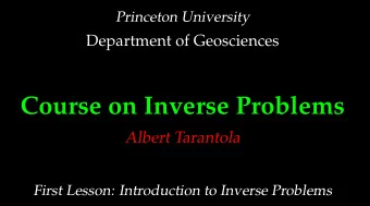
Course on Inverse Problems Albert Tarantola Lesson XV: Square Root - PowerPoint PPT Presentation

Institut de Physique du Globe de Paris & Université Pierre et Marie Curie (Paris VI) Course on Inverse Problems Albert Tarantola Lesson XV: Square Root Variable Metric Algorithm

The Square Root Variable Metric Algorithm for Least-Squares Problems Albert Tarantola 1 Introduction In the context of least-squares, there is an a priori probability distribution on the model parameter space: a Gaussian distribution, with mean m prior and covariance C prior . The result of measuring the observ- able parameters is also expressed with a Gaussian probability distribution, with mean o obs and covari- ance C obs . If the relation m �→ o = o ( m ) predicting the observations that should correspond to model m is not too strongly nonlinear, then, the a posteriori probability distribution in the model space is — approximately— Gaussian. The first numerical problem to solve is that of computing the mean m post and the covariance C post of this posterior Gaussian distribution. The second numerical problem is to obtain samples of that distribution.

2 Misfit Function The model m post , center of the posterior Gaussian distribution, is the model minimizing the misfit function (sum of squares) 2 S ( m ) = � o ( m ) − o obs � 2 + � m − m prior � 2 , (1) where � o ( m ) − o obs � 2 = ( o ( m ) − o obs ) t C -1 obs ( o ( m ) − o obs ) (2) and � m − m prior � 2 = ( m − m prior ) t C -1 prior ( m − m prior ) . (3)

3 Partial Derivatives Gradient methods of optimization require the computation of the matrix O of partial derivatives ∂ o i O i α = . (4) ∂ m α This computation is sometimes performed analytically, as in sin ( t 0 ) ′ = cos ( t 0 ) , (5) sometimes numerically, as in sin ( t 0 ) ′ ≈ sin ( t 0 + ∆ t ) − sin ( t 0 − ∆ t ) ∆ t = 0.001 ; . (6) 2 ∆ t

4 Newton Algorithm When the computer is big enough, the (quasi) Newton algorithm can be implemented. It is then the better choice. The model m post , center of the posterior Gaussian, is obtained as the convergence point of the algo- rithm prior ) -1 ( O t m k + 1 = m k − ( O t k C -1 obs O k + C -1 k C -1 obs ( o ( m k ) − o obs ) + C -1 prior ( m k − m prior ) ) , (7) while the covariance of the posterior Gaussian is the value, at the convergence point, of the matrix C post = ( O t C -1 obs O + C -1 prior ) -1 . (8)

5 Square Root Variable Metric Algorithm 5.1 Introduction In differential geometry, when one considers a manifold with some coordinates { x 1 , x 2 . . . x n } , and the square of length element is written ds 2 = g ij dx i dx j (9) (implicit sum over the indices assumed), one calls the matrix with elements g ij the metric of the mani- fold. If it is a linear manifold, then, the square of the finite distance between two points can be written s 2 = g ij ( x i 2 ) ( x j 1 − x j 1 − x i 2 ) , (10) or, using, obvious matrix notations, s 2 = ( x 1 − x 2 ) t g ( x 1 − x 2 ) . (11) In least-squares theory, we have expressions like D 2 = ( m 1 − m 2 ) t C -1 ( m 1 − m 2 ) , (12) where C is a covariance matrix. These expressions are also to be interpreted as corresponding to a squared distance. We thus see that the inverse of a covariance matrix (a weight matrix) can be considered to define a metric (over the model parameter space) 1 . The variable methods aim at starting using as metric the inverse of the prior covariance matrix, and

to define a metric (over the model parameter space) . The variable methods aim at starting using as metric the inverse of the prior covariance matrix, and making it evolve so at the end we are using as metric the inverse of the posterior covariance matrix. These methods have a rapid convergence, similar to the conjugate directions methods, but have a ad- vantage over them: that of providing a direct estimation of the posterior covariance matrix, say C post . There are two kinds of variable metric algorithms. While the first kind (variable metric algorithms) aim at directly producing C post the second kind (square root variable metric algorithms) aim at produc- ing the square root of C post , say T post . One then has C post = T post T t (13) post (so one can formally write T post = � C post ). The interest in having the square root of the posterior covariance matrix arises from the property that if a vector x is a sample vector of a Gaussian distribution with zero mean and unit covariance matrix, then the vector m = m post + T post x (14) 1 When considering as metric the inverse of the prior covariance we arrive to the steepest descent method, while when consid- ering as metric the inverse of the posterior covariance we arrive to the Newton method.

is a sample vector of a Gaussian distribution with mean m post and covariance C post , i.e., a sample vector of the (approximate) posterior distribution in the model parameter space 2 . In what follows, let us denote by T prior the square root of the prior covariance matrix, C prior = T prior T t . (15) prior The algorithm is initialized at some values m 0 and T 0 that are the best approximations available of the posterior model and the posterior covariance, m 0 ≈ m post ; T 0 ≈ T post . (16) Typically there is no better approximation than the prior values, and one then takes m 0 = m prior ; T 0 = T prior . (17) The square root variable metric algorithm is 3 (other possible algorithms differ only in details): For k = 0, 1, 2 . . .

γ k = C -1 prior ( m k − m prior ) + G t k C -1 obs ( o ( m k ) − o obs ) φ k = T k T t k γ k φ k = C -1 � prior φ k b k = G k φ k � b k = C -1 obs b k γ t k φ k µ k = k � φ t k � φ k + b t b k m k + 1 = m k − µ k φ k (18) φ k + G t k � g k = µ k ( � b k ) y k = µ k γ k − g k w k = T t k y k a k = w t k T t k g k b k = w t k w k c k = 1 − √ 1 + b k / a k b k T k + 1 = T k ( I − c k w k w t k ) .

As already indicated, T k T t m k → m post k → C post ; . (19) 2 Quick and dirty demonstration: the mean of m is m = ( m post + T post x ) = m post + T post x = m post + T post x = m post + = ( m − m post ) ( m − m post ) t = ( T post x ) ( T post x ) t = T post x x t T t T post 0 = m post and the covariance matrix of m is C post = T post x x t T t post = T post I T t post = T post T t post . 3 Williamson, W.E., 1975, Square-root variable metric method for function minimization, AIAA journal, 13 (1), 107–109. Morf, M., and T. Kailath, 1975, Square-root algorithms for least-squares estimation, IEEE Transactions on automatic control, Vol. AC-40, No. 4, 487–497. Hull, D.G., and B.D. Tapley, 1977, Square-root variable-metric methods for minimization, J. Optim. App., Vol. 21, No. 3, 251–259.

The linear form γ k is the gradient of the misfit function at iteration m k . The vector φ k is the direction of search. The scalar µ k defines a reasonable step length (along that search direction). The linear form g k is, in fact the difference between two consecutive gradients 4 . For small-sized problems, the matrices T k can be built. For large-sized problems, those matrices would be too large to store in the computer. The matrix C post would be too large too. (This is typically not true for C prior of for T 0 ≈ � C prior , as we often have analytical expressions for them.) It is then very importat to realize that the only “objects” to be computed (and stored in the computer’s memory) are the constants c 0 , c 1 , c 2 . . . and the vectors w 0 , w 1 , w 2 . . . . With these constants and these vectors, the result of the action of any of the T k on any vector can be computed. For instance, given a vector v , how do we compute the vector ψ = T 1 v ? (20)

The last of equations 18 tells us that T 1 = T 0 ( I − c 0 w 0 w t 0 ) . (21) We have the constant c 0 and the vector w 0 , and the operator T 0 is assumed to be simple enough (typically, T 0 = I , or T 0 is chosen so that it has an analytical expression). Then, ψ = T 1 v = T 0 ( I − c 0 w 0 w t 0 ) v = T 0 ( v − c 0 w 0 w t 0 v ) (22) = T 0 ( v − c 0 ( w t 0 v ) w 0 ) . � �� � scalar This computation only requires the handling of vectors (and of the operator T 0 that is assumed to be a simple one). Applying this notion recursively, we can compute the action of any of the T k on any vector v k : ψ k = T k v k . (23) Notably, this will apply when, after convergence of the square root variable metric algorithm, we face the task of generating samples of the posterior Gaussian, via expression 14.

4 g k = γ k − γ k + 1 = C -1 prior ( m k − m prior ) + G t k C -1 obs ( o ( m k ) − o obs ) − C -1 prior ( m k + 1 − m prior ) − G t k + 1 C -1 obs ( o ( m k + 1 ) − o obs ) ≈ C -1 prior ( m k − m prior ) + G t k C -1 obs ( o ( m k ) − o obs ) − C -1 prior ( m k + 1 − m prior ) − G t k C -1 − C -1 obs ( o ( m k + 1 ) − o obs ) = prior ( m k + 1 − m k ) − G t k C -1 − C -1 prior ( m k + 1 − m k ) − G t k C -1 − ( C -1 prior + G t k C -1 obs ( o ( m k + 1 ) − o ( m k )) = obs G k ( m k + 1 − m k ) = obs G k ) ( m k + 1 − m k ) = k � µ k ( C -1 prior + G t k C -1 obs G k ) φ k = µ k ( � φ k + G t b k ) .