Inverse Kinematics Inverse Kinematics Inverse Kinematics Carnegie - PowerPoint PPT Presentation
Inverse Kinematics Inverse Kinematics Inverse Kinematics Carnegie Carnegie Sebastian Grassia Sebastian Grassia Mellon Mellon School of Computer Science School of Computer Science Define the Problem Define the Problem Define the Problem
Inverse Kinematics Inverse Kinematics Inverse Kinematics Carnegie Carnegie Sebastian Grassia Sebastian Grassia Mellon Mellon School of Computer Science School of Computer Science
Define the Problem Define the Problem Define the Problem follow mouse follow mouse p p 1 1 Goals Goals • Drag in realtime with mouse Drag in realtime with mouse • • Maintain multiple constraints Maintain multiple constraints • • Figure responds in “reasonable” Figure responds in “reasonable” ways ways • p p p p 2 2 3 3 Stay put Stay put
... Then Name the System! ... Then Name the System! ... Then Name the System! p p 1 1 Use standard transformation hierarchy Use standard transformation hierarchy root root p 1 = T ( x , y , z ) R ( θ , φ , ϕ ) TR ( γ )... TR ( σ ) p b q ( t ) = ... ... p 1 = C ( q ( t ) ) p p p p 2 2 3 3
Idea #1 Idea #1 Idea #1 Let Let p m ( t ) = p m ( t ) = 3D mouse positioner at time t t 3D mouse positioner at time C ( q ( t ) ) = C ( q ( t ) ) = position of hand at time t t position of hand at time such that q ... then solve for then solve for q such that ... C ( q ( t ) ) = p m ( t ) C ( q ( t ) ) = p m ( t )
Unfortunately... Unfortunately... Unfortunately... C ( q ( t ) ) = p m ( t ) C ( q ( t ) ) = p m ( t ) contains rotations, therefore nonlinear, contains rotations, therefore nonlinear, and very difficult to solve and very difficult to solve Can be solved for: Can be solved for: • articulated chains articulated chains • Has real problems with: Has real problems with: • branching hierarchies branching hierarchies • • multiple constraints multiple constraints • • convincing motion convincing motion •
Idea #2 Idea #2 Idea #2 Let’s differentiate! Let’s differentiate! ∂ ∂ ( ) ( ) ∂ t p m ( t ) = C ( q ( t ) ) ∂ t p m ( t ) = C ( q ( t ) ) m = ∂ C m = ∂ C p ˙ ∂ q ˙ q p ˙ ∂ q ˙ q desired – actual desired – actual state space velocity state space velocity J Jacobian J Jacobian
A Diffy Q by any other name... A Diffy Q by any other name... A Diffy Q by any other name... p = J ˙ p = J ˙ ˙ q ˙ q = Underdetermined linear system p ˙ = Underdetermined linear system p ˙ J J q ˙ q ˙ Can solve for Can solve for . . . . . q ˙ . . q ˙ . . . . . Iterate during interaction using: Iterate during interaction using: q ( t + ∆ t ) = q ( t ) + ∆ t ˙ q ( t + ∆ t ) = q ( t ) + ∆ t ˙ q ( t ) q ( t )
Are we there yet? Are we there yet? Are we there yet? Alas, no. Alas, no. We got a a solution for solution for We got q ˙ q ˙ but it may not be a reasonable reasonable one. one. but it may not be a Why not? Why not?
Scaling Scaling Scaling When there’s a choice, When there’s a choice, radians radians least squares solver always least squares solver always moves shoulder before elbow moves shoulder before elbow degrees degrees Measuring both angles in radians Measuring both angles in radians still leaves figure stiff-armed still leaves figure stiff-armed What can we do about this? What can we do about this?
Let’s get physical! Let’s get physical! Let’s get physical! Aristotlean physics: Aristotlean physics: f = Mv f = Mv f = Ma f = Ma ? ? Why not Why not f G + f C = M ˙ f G + f C = M ˙ q q Generalized Force Generalized Force Mass Matrix Mass Matrix Constraint Force Constraint Force
Blend on High for 2 minutes... Blend on High for 2 minutes... Blend on High for 2 minutes... Recall Recall Constraints Constraints f G + f C = M ˙ f G + f C = M ˙ q q p = C ( q ) p = C ( q ) Lagrange Multipliers Lagrange Multipliers Solve Solve p = J ˙ p = J ˙ ˙ q ˙ q f G + J T λ = M ˙ f G + J T λ = M ˙ q q substitute substitute J = ∂ C J = ∂ C Where Where ( ) ( ) get get q = W f G + J q = W f G + J ∂ q ∂ q T λ T λ ˙ ˙ − 1 W = M − 1 Define: W = M p = JWf G + JWJ Define: p = JWf G + JWJ T λ T λ ˙ ˙
Recalling Lagrange Multipliers Recalling Lagrange Multipliers Recalling Lagrange Multipliers Then... Then... f C = λ N Assumption of passive passive constraints constraints Assumption of f C f C stipulated that point along stipulated that point along ∂ C ∂ C ∂ x = N ∂ x = N constraint gradient constraint gradient Now... Now... ∂ C ∂ C ∂ q = J ∂ q = J Constraint gradients: Constraint gradients: Point-on-circle Point-on-circle f C is a f C is a linear combination linear combination of of constraint gradients: constraint gradients: C ( x ) = x − r = 0 C ( x ) = x − r = 0 f C = J T λ
and wind up with: and wind up with: and wind up with: p − JWf G = JWJ p − JWf G = JWJ T λ T λ ˙ ˙ = = λ λ J J W W T T J J λ , plug into formula for Can solve for λ q ˙ , plug into formula for ˙ q Can solve for
Have we solved the scaling problem? Have we solved the scaling problem? Have we solved the scaling problem? We get a velocity that obeys q ˙ We get a velocity that obeys q ˙ f = Mv f = Mv the “physical law” ... the “physical law” ... M M determines how the system responds determines how the system responds to applied forces. to applied forces. So it all depends on what is. M is. So it all depends on what M
How well can we do? How well can we do? How well can we do? If approximate figure by rigid, If approximate figure by rigid, uniform density, simple shapes... uniform density, simple shapes... M ( q ) M ( q ) Can derive and compute an Can derive and compute an from minimizing kinetic energy from minimizing kinetic energy of articulated figure of articulated figure Minimum energy consumption is good! Minimum energy consumption is good!
A word about J A word about J A word about J p p p only depends on ancestors p only depends on ancestors 1 1 1 1 in hierarchy in hierarchy J J Therefore, is sparse. Exact is sparse. Exact Therefore, root root pattern depends on ordering pattern depends on ordering q . of q . of Can compute all derivatives Can compute all derivatives efficiently in recursive efficiently in recursive tree traversal tree traversal
What’s in the online notes What’s in the online notes What’s in the online notes • More detailed derivations More detailed derivations • • Formula for computing Mass Matrix Formula for computing Mass Matrix • • Pseudocode for tree traversal Pseudocode for tree traversal • • Bibliography Bibliography •
That’s Just the Beginning... That’s Just the Beginning... That’s Just the Beginning... → joint limits One sided constraints → • One sided constraints joint limits • • Hierarchical constraints Hierarchical constraints • • Spring “muscles” Spring “muscles” • • Build complex constraint functions for Build complex constraint functions for • higher level behavior higher level behavior
Recommend
More recommend
Explore More Topics
Stay informed with curated content and fresh updates.
