Course on Inverse Problems Albert Tarantola First Lesson: - PowerPoint PPT Presentation

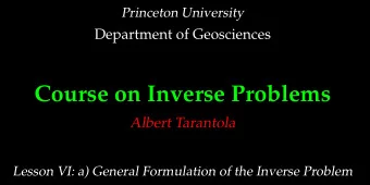
Princeton University Department of Geosciences Course on Inverse Problems Albert Tarantola First Lesson: Introduction to Inverse Problems

The Bayes-Popper approach. Using observations to infer the values of some parameters cor- responds to solving an inverse problem . Practitioners some- times seek the best solution implied by the data, but observa- tions should only be used to falsify possible solutions, not to deduce any particular solution.

Name frequency Åland Albania Aleutian Islands Algeria American Samoa Andorra Angola . . . States, Territories, and Principal Islands of the World first digit Benford model actual statistics 1 . . . 2 3 4 5 6 7 8 9 0 400 300 200 Afghanistan 6 ,920,000 Sq. km 5 81 Sq. miles Population 6 36,267 1 ,505 2 8,748 1 7,666 2 ,381,745 1 97 4 65 1 ,246,700 . . . 2 45,664 1 1,097 3 5,460 6 ,821 9 19,354 7 6 1 80 4 81,226 . . . 1 5,551,358 2 2,000 2 ,590,600 6 ,730 1 8,250,000 3 0,600 100

speed of light in vacuum 6 frequency 1 2 3 4 5 7 Benford model 8 9 80 60 40 20 actual statistics first digit . . . G = 6 .673(10) 10 -11 m 3 kg -1 s -2 Newtonian constant of gravitation Planck constant elementary charge . . . c = 2 99 792 458 m s -1 . . . h = 6 .626 068 76(52) 10 -34 J s CODATA recommended values of the fundamental physical constants = 4 .135 667 27(16) 10 -15 eV h = 1 .054 571 596(82) 10 -34 J s = 6 .582 118 89(26) 10 -16 eV e = 1 .602 176 462(63) 10 -19 C e / h = 2 .417 989 491(95) 10 14 A J -1 . . . 0

2 10 X = 10 x 0.2 0.5 0.1 1 2 5 20 1.5 50 100 -1 -0.5 0 0.5 1 x = log 10 X

infinitely resisting wires infinitely conducting wires which is the distance between two electric wires? (spaces that represent physical qualities) physical quantities are coordinates over abstract spaces c = 1 c = 2 c = - 2 c = - 1 c = 0 r = - 1 r = - 2 r = 2 r = 1 r = 0 = | dc| space of electric wires: C = 1 S R = 1 Ω R = e Ω R = e 2 Ω R = 1/ e Ω = | dr| R = 1/ e 2 Ω C = 1/ e S C = 1/ e 2 S C = e S C = e 2 S given two wires W 1 and W 2 , which is the average wire? d l = | dR |/ R W 1 W 2 d l d l = | dC |/ C

C8 - 4186.0 Hz - 238.89 µ s B7 - 3951.1 Hz - 253.10 µ s A7# - 3729.3 Hz - 268.15 µ s A7 - 3520.0 Hz - 284.09 µ s G7# - 3322.4 Hz - 300.98 µ s G7 - 3136.0 Hz - 318.88 µ s F7# - 2960.0 Hz - 337.84 µ s F7 - 2793.8 Hz - 357.93 µ s E7 - 2637.0 Hz - 379.22 µ s D7# - 2489.0 Hz - 401.76 µ s D7 - 2349.3 Hz - 425.65 µ s C7# - 2217.5 Hz - 450.97 µ s C7 - 2093.0 Hz - 477.78 µ s B6 - 1975.5 Hz - 506.19 µ s A6# - 1864.7 Hz - 536.29 µ s A6 - 1760.0 Hz - 568.18 µ s G6# - 1661.2 Hz - 601.97 µ s G6 - 1568.0 Hz - 637.76 µ s F6# - 1480.0 Hz - 675.69 µ s F6 - 1396.9 Hz - 715.86 µ s E6 - 1318.5 Hz - 758.43 µ s D6# - 1244.5 Hz - 803.53 µ s D6 - 1174.7 Hz - 851.31 µ s C6# - 1108.7 Hz - 901.93 µ s C6 - 1046.5 Hz - 955.56 µ s B5 - 987.77 Hz - 1012.3 µ s A5# - 932.33 Hz - 1072.5 µ s A5 - 880.00 Hz - 1136.4 µ s G5# - 830.61 Hz - 1203.9 µ s G5 - 783.99 Hz - 1275.5 µ s F5# - 739.99 Hz - 1351.4 µ s F5 - 689.46 Hz - 1431.7 µ s E5 - 659.26 Hz - 1616.9 µ s D5# - 622.25 Hz - 1607.1 µ s D5 - 587.33 Hz - 1702.6 µ s C5# - 554.37 Hz - 1803.9 µ s C5 - 523.25 Hz - 1911.1 µ s B4 - 493.88 Hz - 2024.8 µ s A4# - 466.16 Hz - 2145.2 µ s A4 - 440.00 Hz - 2272.7 µ s G4# - 415.30 Hz - 2407.9 µ s G4 - 392.00 Hz - 2551.0 µ s F4# - 369.99 Hz - 2702.7 µ s F4 - 349.23 Hz - 2863.5 µ s E4 - 329.63 Hz - 3033.7 µ s D4# - 311.13 Hz - 3214.1 µ s D4 - 293.66 Hz - 3405.2 µ s C4# - 277.18 Hz - 3607.7 µ s C4 - 261.63 Hz - 3822.3 µ s

A musical note N can be characterized, for instance, by the frequency ν or by the period T . Which is the distance between two musical notes N 1 and N 2 ? | = | log T 1 D ( N 1 , N 2 ) = | log ν 1 | ν 2 T 2

33฀1/3 45

Examples of Jeffreys quantities frequency ν = 1 period τ = 1 − τ ν wevelength λ = 1 wavenumber κ = 1 − κ λ temperature T = 1 thermodynamic parameter β = 1 − k β k T

ρ = 10 g/cm 3 ρ = 20 g/cm 3 ρ = 0 r = 0 r = 0.5 r = 1 r = 1.5 r = log 10 ( ρ / ρ 0 ) ( ρ 0 = 1 g/cm 3 ) ∆ρ/ρ฀ constant ⇒ volumetric probability f ( ρ ) ∆ρ฀ constant ⇒ probability density f ( ρ ) _ ρ = 1 g/cm 3 ρ = 3.2 g/cm 3 ρ = 10 g/cm 3 ρ = 32 g/cm 3