Continuum Branching Observable in Higher Genus (Based on Discussion - PowerPoint PPT Presentation
Continuum Branching Observable in Higher Genus (Based on Discussion with Nicolai Reshetikhin) Matthew Bernard mattb@berkeley.edu Advanced Computational Biology Center , Berkeley Supported by The Lynn Bit Foundation , State of California
Continuum Branching Observable in Higher Genus (Based on Discussion with Nicolai Reshetikhin) Matthew Bernard mattb@berkeley.edu Advanced Computational Biology Center , Berkeley Supported by The Lynn Bit Foundation , State of California
Abstract 2 We prove : R -valued partition invariant in supersymmetry for all fjxed suffjcient large genus g ⩾ 0 multiedge embedding ; and , the O ( n 3 ) bipartite observable in Grassmann kernel transfer matrices on discrete functions for all spanning dual trees . In special hexagonal domain , we prove the free Dirac Fermion convergence Ψ= f · (1 + O (1)) on logarithmic discriminant steepest descent of Grassmann kernel asymptotics . We conjecture : In large deviation , Green’s function G for Dirichlet problem of variational principle minimizer is observable in the kernel asymptotics . Keywords: Continuum-branching , Higher-genus , Observable
1 Characterizations for triangular grids 3 • ◦ Bipartite implies no adjacent-black (-white) vertices for all V X = V X ⊔ V X : M × N vertices , ( M − 1) × ( N − 1) path cartesian latticial edges ; 2 n = MN. Instance . 1 6 12 18 1 2 3 4 2 7 13 19 24 3 8 14 20 25 5 6 7 8 4 9 15 21 26 5 10 16 22 27 9 10 11 12 . 11 17 23 28 Non-instance . 1 2 3 4 � no bipartite structure � . 5 6 7 8 9 10 11 12
1.1 Partition function on topological embedding 4 ∀ g ≫ , an embedding X ⊂ M g | V X = ( i ℓ ; i ℓ = i ξ � = j ℓ , ∀ i � = j ) is partition σ ∈ Aut ( D ) ⇐ ⇒ perfect-matching D ⇐ ⇒ | i ℓ ∩ D | = 1 , ∀ i ℓ ∈ V X , and � ℓ � = ξ ∈ D ( i ℓ , j ξ ) = ∅ ; for D =( D, ∀ ℓ ); M g orientable compact , X closed ; 1 6 2 5 7 8 3 4 � � � equals � � ∂D = V i.e ., 1 ℓ � = ξ σ D ( i ℓ j ℓ ) defjned as : X 2 � � � � 1 if ℓ ∈ D Aut ( D ) | − 1 | Aut ( D ) | · | σ � � � = 0 ⇐ ⇒ ( i ℓ , j ξ ) � = ∅ � σ D ( i ℓ j ℓ )= exp { n ln 2 + � n − 1 0 if ℓ �∈ D k =2 ln k } ℓ � = ξ ∈ D X = ( i ℓ | i =1 , . . . , 2 n ; ∀ n ⩽ | ℓ | < ∞ , n ∈ N + ) , and for all V X ⊂ M g is CW cell-complex i.e . face ≈ topological disk i.e . no hole .
5 2 4 2 1 3 5 1 3 6 8 10 7 9 0 0 0 0 0 0 0 1 1 0 0 1 1 1 0 0 4 6 0 0 0 0 0 0 0 0 0 0 0 0 0 0 0 0 0 0 0 1 0 1 1 1 1 1 1 1 1 1 1 1 1 1 1 0 1 0 0 0 0 0 0 0 0 0 0 0 0 0 0 0 1 1 1 1 1 1 1 1 1 1 1 1 1 1 1 1 1 1 1 1 1 1 1 1 0 0 0 0 0 0 0 0 0 0 0 0 0 0 0 0 1 0 1 0 0 1 1 1 0 0 1 1 1 1 1 1 0 1 1 0 0 0 0 0 1 0 0 1 1 1 1 1 1 1 0 0 0 0 0 0 0 0 0 0 0 0 0 0 0 0 1 1 1 1 1 1 1 1 1 1 1 1 1 1 1 1 1 1 1 1 1 1 1 1 0 0 0 0 0 0 0 0 0 0 0 0 0 0 0 0 5 1 1 0 1 1 1 1 1 1 1 1 1 1 1 1 1 1 1 1 1 1 1 1 1 1 1 0 0 0 0 0 0 1 0 0 1 1 1 1 1 1 1 1 1 1 1 1 1 1 1 1 1 1 1 1 1 1 1 1 1 1 1 1 1 1 1 1 1 1 1 1 1 1 1 1 1 1 1 1 1 1 1 1 1 1 1 1 1 1 1 0 1 1 1 1 1 0 0 0 0 1 1 1 1 1 1 1 1 1 1 1 1 1 1 1 1 1 1 1 1 . 0 0 0 0 1 1 1 1 1 1 1 1 1 1 1 1 1 1 1 1 1 1 1 1 0 0 1 0 1 0 0 1 1 1 0 0 0 0 0 0 0 0 0 0 0 0 0 0 0 1 0 1 1 1 1 1 1 1 0 0 0 0 0 0 0 0 1 1 1 1 1 1 1 1 0 0 0 0 0 0 0 0 0 0 0 0 0 0 1 0 0 1 1 1 1 1 1 1 1 1 1 1 1 1 1 1 1 1 1 1 1 1 1 1 1 1 1 1 1 0 0 0 0 0 1 1 1 1 1 1 1 1 1 1 1 1 1 1 1 1 1 1 1 1 1 1 1 1 0 0 1 0 0 1 1 1 1 1 1 1 1 1 1 1 1 1 1 1 0 0 1 1 0 0 0 1 1 1 0 0 0 0 0 0 0 0 1 1 1 1 1 1 1 1 0 0 0 0 0 0 0 0 0 0 0 0 1 1 1 1 1 1 1 1 1 1 1 1 0 0 0 0 0 0 0 0 1 1 1 1 1 1 1 1 0 0 0 0 0 0 0 0 0 0 0 0 1 1 1 1 1 1 1 1 1 1 1 1 1 1 1 1 1 1 1 1 1 1 0 0 0 0 0 1 1 1 1 1 1 1 1 1 1 1 1 1 1 1 1 1 1 1 1 1 1 1 0 0 0 0 1 1 1 1 1 1 1 1 1 1 1 1 1 1 1 1 1 1 1 1 1 1 1 1 1 1 1 0 0 0 0 0 0 0 0 0 0 0 0 0 0 0 1 1 1 1 1 1 1 1 1 1 0 0 0 0 0 0 0 0 0 0 1 1 1 1 1 1 1 1 1 1 1 1 0 0 0 0 0 0 0 0 0 0 0 0 1 1 1 1 1 1 1 1 0 0 0 0 0 0 0 0 1 1 1 1 1 1 1 1 1 1 1 1 1 1 1 0 0 0 0 0 1 1 1 1 1 1 1 1 1 1 1 1 1 1 1 1 1 1 1 1 1 1 0 0 0 0 1 1 1 1 1 1 1 1 1 1 1 0 0 1 0 1 0 0 1 1 1 1 1 1 1 1 1 1 1 1 1 1 1 1 1 1 1 1 1 1 1 1 0 0 0 0 0 0 0 0 0 0 0 0 0 0 0 0 1 1 1 1 1 1 1 1 0 0 0 0 0 0 1 0 0 1 1 1 1 1 1 0 1 0 0 0 0 0 0 0 0 0 0 0 0 0 0 0 1 1 1 1 1 1 1 1 1 1 1 1 1 1 1 1 1 1 1 1 0 0 0 0 0 1 1 1 1 1 1 1 1 1 1 1 1 1 1 1 1 1 1 1 1 1 0 0 0 0 1 1 1 1 1 1 1 1 1 1 1 0 1 1 1 1 1 1 1 1 1 1 1 1 1 1 1 1 1 1 1 1 1 1 1 1 1 1 1 1 1 1 1 1 1 1 1 1 1 1 1 1 1 1 1 1 1 1 1 1 1 1 1 1 1 1 1 1 1 1 0 0 0 0 0 0 0 0 1 1 1 1 1 1 1 1 1 1 1 1 1 1 1 1 1 1 1 1 1 0 1 1 1 1 1 1 1 1 1 1 1 1 1 1 1 1 1 1 1 1 1 1 1 1 1 1 1 1 1 1 1 1 1 1 1 1 1 1 1 0 1 0 0 0 0 0 0 0 0 0 1 1 1 0 0 1 0 1 0 0 0 0 0 0 0 0 0 0 0 0 0 0 1 0 0 1 1 1 1 1 1 1 1 1 1 1 1 1 1 1 1 1 1 1 1 1 1 1 0 0 0 0 0 0 0 0 0 0 0 0 0 0 0 1 0 1 1 1 1 1 1 1 0 0 0 0 0 0 0 0 1 1 1 1 1 1 1 1 0 ( σ D ( i ℓ j ℓ )) := 0 0 0 0 0 0 ⇐ ⇒ ℓ �∈ D , 0 0 0 0 1 1 1 0 0 1 1 0 0 0 0 0 0 0 0 0 0 0 0 0 0 0 0 1 0 1 1 1 1 1 1 1 1 1 1 1 1 1 1 1 1 1 1 1 1 1 1 1 0 0 0 0 0 0 0 0 0 0 0 0 0 0 0 1 0 1 1 1 1 1 1 1 1 1 1 1 1 1 1 1 0 0 0 0 0 0 0 0 1 1 1 & 1 1 1 1 1 1 1 1 , 1 1 1 1 1 1 , 1 1 1 1 1 1 1 1 1 1 ⇐ ⇒ ℓ ∈ D .
6 � � � 2 )) ∼ ∼ ( Aut ( D ) / ( S n ×S n = { � = σ σ } Aut ( D ) } ∼ � = ( S n ×S n Aut ( D ) Derivation. (i) { σ 2 ) � (2 n )! · 2 − ((1 / ε ) mod c ( X K )) · e ln ( a ( X K ) · b ( X K )) � 1 / (2 | D | ) σ }| 1 / | D | ⩽ (ii) |{ � � n ! · a ( X K ) · b ( X K ) � � a, b, c ∈ R + ; n ⩾ 2; for min(deg( X K )) ⩾ ⌊ 2 n − 3 ⌋ !! = � ⌊ n ⌋− 2 2 k +1 k =0 − X K ∋ σ :=( σ (1) , . . . , σ (2 n )); � Im ( Aut ( D )) ← σ = σ | σ (2 ℓ ) > σ (2 ℓ − 1); S n := { ( σ (1) , . . . , σ (2 n )) , . . . , ( σ (2 n − 1) , σ (2 n ) , . . . , σ (1) , σ (2)) } S n 2 := { ( σ (1) , . . . , σ (2 n )) , . . . , ( σ (2) , σ (1) , . . . , σ (2 n ) , σ (2 n − 1)) } for objects : 1 2 3 4 6 11 30 1 14 15 5 6 7 8 66 5 10 19 29 2 13 16 9 10 11 12 • Square grid domains . 4 9 • (regular) Hexagonal grid domains .
7 correlation (conditional probability) equals def By E [ σ D ( i ℓ j ℓ ) σ D ( i ξ j ξ )] = E [ σ D ( i ℓ j ℓ )] ⇐ ⇒ ℓ = ξ , resp . 0 ⇐ ⇒ σ D ( i ℓ j ℓ ) = 0 or ( i ℓ j ℓ ) , ( i ξ j ξ ) | ℓ � = ξ share vertex : The local observable i.e . dimer-dimer � k � � � k � � σ D ( i ℓ j ℓ ) = = Prob ( i 1 j 1 ∈ D, . . . , i k j k ∈ D ) = E σ D ( i ℓ j ℓ ) ℓ = 1 ℓ = 1 � � σ D ( i ℓ j ℓ ) � k ω ℓ k � � D ∈ D ℓ = 1 ℓ ∈ D � � σ D ( i ℓ j ℓ ) × Prob ( D ) = ω ℓ D ∈ D ℓ = 1 ℓ ∈ D D ∈ D � � � ⇒ 1 Ξ ( · ) � e − � = 0 ⇐ ω D � K T , ω ( · ) = Ξ ( · ) = Ξ ℓ � Z � D ∋ ( i 1 j 1 ) , ..., ( i k j k ) ℓ ∈ ( · ) ℓ ∈ ( · ) � � � � � � � � � Z def = = ω ℓ = Prob ( D ) ⇐ ⇒ = ∅ D ( i ℓ j ℓ ) � D ∈ D ℓ ∈ D D ∈ D for strict-sense positive partition function Z on Boltzmann weights ω ( · ) by → R + | ℓ �− X − → Ξ ℓ . Ξ : E
1.2 (i) Measure-preserving notion of spanning dual trees 8 Proposition (combinatorial-equivalence). Given a dimer space (resp . tiling space) , there exits one-to-one combinatorial correspondence: → family (Tilings) . family (Dimers) ← Proof . Let X ⊂ R 2 be planar (no intersected edge) orientable . That is , 2 D cell complex on X (union of all spanning trees T ) : 0 -cells , 1 -cells , 2 -cells = vertices , edges , faces , resp . 1 12 11 Disjoint interiors . 2 3 10 4 7 dim( ∂X ( k ) ) = ( k − 1) mod 2 9 ∂X ( k ) = boundary of two k -cells , 14 13 k = 0 , 1 , 2 . 5 6 8 Remark . X ⊂ M g is generally , 1 -skeleton CW-complex (resp. orientable , compact genus g cell-decomposition) .
(ii) cell complex 9 2 D dual cell complex on X ∗ (union of all spanning dual trees T ∗ ) : 0 -cells , 1 -cells , 2 -cells = resp . “ centers ” of 2 -cells , 1 -cells , 0 -cells of X : 1 12 11 22 23 21 X ∗ = dual 2 3 10 25 15 27 4 7 18 to X. 16 9 13 14 26 19 5 17 6 8 Unique pair of 2 -cells on X ∗ share : (iii) For a dimer on X : 1 1 11 11 22 23 21 2 2 3 3 10 10 25 15 4 4 7 7 (iv) Therefore , the global bijection : � Tilings of X ∗ by � (Dimers on X ) . □ ← → unique pair of 2 -cells
Recommend
More recommend
Explore More Topics
Stay informed with curated content and fresh updates.
