1 Stochastic, Partially Observable Markov Decision Process (MDP) - PowerPoint PPT Presentation
Stochastic Planning Classical Planning (MDPs, Reinforcement Learning) Static Predictable Unpredictable Static CSE 473 Artificial Intelligence Environment Environment Fully Fully Observable Discrete Observable Observable Discrete
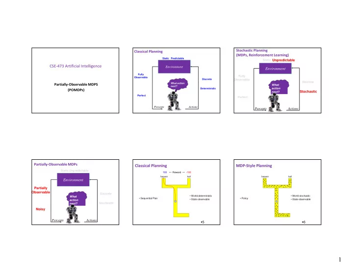
Stochastic Planning Classical Planning (MDPs, Reinforcement Learning) Static Predictable Unpredictable Static CSE ‐ 473 Artificial Intelligence Environment Environment Fully Fully Observable Discrete Observable Observable Discrete What action Partially ‐ Observable MDPS What next? action Deterministic (POMDPs) Stochastic next? Perfect Perfect Percepts Actions Percepts Actions Partially ‐ Observable MDPs Classical Planning MDP ‐ Style Planning Static Unpredictable 100 Reward -100 heaven hell heaven hell Environment Partially Observable Observable Discrete • World deterministic • World stochastic What • Sequential Plan • Policy • State observable • State observable action Stochastic next? Noisy Percepts Actions 5 6 1
Stochastic, Partially Observable Markov Decision Process (MDP) Partially ‐ Observable MDP S : S : set of states set of states heaven? hell? A : A : set of actions set of actions P r(s’|s,a): transition model P r (s’|s,a): transition model R (s,a,s’): reward model R (s,a,s’): reward model : : discount factor discount factor s 0 : s 0 : start state start state E set of possible evidence (observations) P r (e|s) sign 7 Belief State Planning in Belief Space Partially ‐ Observable MDP State of agent’s mind For now, assume movement is Not just of world deterministic S : set of states sign sign A : set of actions 50% 50% P r (s’|s,a): transition model Exp. Reward: 0 R (s,a,s’): reward model : discount factor N s 0 : start state sign sign sign sign Exp. Reward: 0 50% 50% 50% 50% E set of possible evidence (observations) sign sign P r (e|s) Probs = 1 50% 50% sign sign 50% 50% Note: POMDP 10 2
Pr(heat | s eb ) = 1.0 Evidence Model Planning in Belief Space Objective of a Fully Observable MDP Pr(heat | s wb ) = 0.2 S = {s wb , s eb , s wm , s em s wul , s eul s wur , s eur } Find a policy : S → A E = {heat} P r(e|s): s eb which maximizes expected discounted reward heat Pr(heat | s eb ) = 1.0 sign sign 100% 00% 0% sign g Pr(heat | s wb ) = 0.2 • given an infinite horizon Pr(heat | s other ) = 0.0 S • assuming full observability sign sign 50% 50% s wb heat sign sign sign 17% 83% Planning in HW 4 Objective of a POMDP Best plan to eat final food? Map Estimate Now “know” state Find a policy : BeliefStates( S ) → A Solve MDP A belief state is a probability distribution over states which maximizes expected discounted reward • given an infinite horizon • assuming partial & noisy observability 1 3
Best plan to eat final food? Problem with Planning from MAP Estimate POMDPs In POMDPs we apply the very same idea as in MDPs. Since the state is not observable, the agent has to make its decisions based on the belief state which is a posterior distribution over states. Let b be the belief of the agent about the state under 51% 49% consideration. 90% 10% POMDPs compute a value function over belief space: Best action for belief state over k worlds may not be the best action in any one of those worlds 21 measurements state x 1 action u 3 state x 2 measurements 0 . 2 0 . 8 z z 0 . 7 0 3 . An I llustrative Exam ple 1 u 1 Problem s W hat is Belief Space? x 3 u x z 1 2 3 z 2 0 3 . 0 7 . 2 0 . 8 0 . 2 u u u u 1 2 1 2 actions u 1, u 2 100 100 100 50 Each belief is a probability distribution, thus, each value measurements state x 1 action u 3 state x 2 measurements payoff payoff Value in a POMDP is a function of an entire probability 0 . 2 distribution . 0 . 8 z z 0 . 7 0 . 3 u 1 1 This is problematic, since probability distributions are x 3 x u 1 2 z z 3 3 z z continuous . ti 0 . 3 0 . 7 2 2 0 . 8 How many belief states are there? 0 . 2 u u u u actions u 1, u 2 1 2 1 2 For finite worlds with finite state, action, and 100 100 100 50 measurement spaces and finite horizons, however, we can effectively represent the value functions by payoff payoff piecewise linear functions . P(state= x 1 ) 22 23 24 4
measurements state x 1 action u 3 state x 2 measurements 0 2 . Payoffs in Our Exam ple 0 8 . z 0 7 . 0 . 3 z The Param eters of the Exam ple Payoff in POMDPs u 1 1 x 3 x u z 1 3 2 z 0 . 3 0 . 7 2 2 0 8 . 0 . 2 u u u u actions u 1, u 2 1 2 1 2 The actions u 1 and u 2 are terminal actions. In MDPs, the payoff (or return) I f we are totally certain that we 100 100 100 50 payoff payoff are in state x 1 and execute action u 1 , The action u 3 is a sensing action that potentially depended on the state of the system. we receive a reward of -100 leads to a state transition. In POMDPs, however, the true state is The horizon is finite and = 1. I f, on the other hand, we definitely know that we not exactly known. are in x 2 and execute u 1 , the reward is + 100. Therefore, we compute the expected Therefore we compute the expected I n between it is the linear combination of the I n between it is the linear combination of the extreme values weighted by the probabilities payoff by integrating over all states : = 100 – 200 p 1 25 26 27 measurements state x 1 action u 3 state x 2 measurements 0 . 2 The Resulting Policy for T= 1 Payoffs in Our Exam ple 0 . 8 z z 0 . 7 0 . 3 1 u 1 Payoffs in Our Exam ple ( 2 ) x 3 u x z 1 2 3 z 2 0 . 3 0 . 7 2 0 . 8 0 . 2 Given a finite POMDP with time horizon = 1 u u u u 1 2 1 2 actions u 1, u 2 I f we are totally certain that we 100 100 100 50 Use V 1 (b) to determine the optimal policy. payoff payoff are in state x 1 and execute action u 1 , we receive a reward of -100 I f, on the other hand, we definitely know that we are in x 2 and execute u 1 , the reward is + 100. I n between it is the linear combination of the I n between it is the linear combination of the extreme values weighted by the probabilities Corresponding value: = 100 – 200 p 1 = 150 p 1 – 50 28 29 30 5
Pruning Piecew ise Linearity, Convexity I ncreasing the Tim e Horizon Assume the robot can make an observation before The resulting value function V 1 (b) is deciding on an action. the maximum of the three functions at each point With V 1 (b) , note that only the first two components contribute. p The third component can be safely pruned It is piecewise linear and convex. V 1 (b) 31 32 33 I ncreasing the Tim e Horizon Value Function Expected Value after Measuring What if the robot can observe before acting? V 1 (b) But, we do not know in advance what Suppose it perceives z 1 : p(z 1 | x 1 )=0.7 and p(z 1 | x 2 )=0.3 . the next measurement will be, Given the obs z 1 we update the belief using ...? Bayes rule. So we must compute the expected belief 0 . 7 p p ' 1 where p ( z ) 0 . 7 p 0 . 3 ( 1 p ) 0 . 4 p 0 . 3 1 1 1 1 1 2 p ( z ) 1 V V ( ( b b ) ) E E [ [ V V ( ( b b | | z z )] )] p p ( ( z z ) ) V V ( ( b b | | z z ) ) 1 1 z 1 1 i i 1 1 i i Now, V 1 (b | z 1 ) is given by i 1 2 p ( z | x ) p i 1 1 p ( z ) V i 1 p ( z ) i 1 i 2 V p ( z | x ) p b’(b| z 1 ) 1 i 1 1 i 1 V 1 (b| z 1 ) 34 35 36 6
Expected Value after Measuring Resulting Value Function Value Function The four possible combinations yield the p(z 1 ) V 1 (b| z 1 ) But, we do not know in advance what following function which then can be simplified the next measurement will be, and pruned. So we must compute the expected belief \ bar{ V} 1 (b) b’(b| z 1 ) p(z 2 ) V 2 (b| z 2 ) 37 38 39 State Transitions ( Prediction) Resulting Value Function after executing u 3 Value Function after executing u 3 When the agent selects u 3 its state may change. When computing the value function, we have to take Taking the state transitions into account, we finally obtain. \ bar{ V} 1 (b) these potential state changes into account. \ bar{ V} 1 (b| u 3 ) 40 41 42 7
Deep Horizons Graphical Representation of V 2 (b) Value Function for T= 2 We have now completed a full backup in belief space. This process can be applied recursively. Taking into account that the agent can u 2 optimal u 1 optimal either directly perform u 1 or u 2 or first u 3 and The value functions for T=10 and T=20 are then u 1 or u 2 , we obtain (after pruning) unclear outcom e of m easuring is im portant here 43 44 45 Deep Horizons and Pruning W hy Pruning is Essential POMDP Approxim ations Each update introduces additional linear Point-based value iteration com ponents to V . Each m easurem ent squares the num ber of linear com ponents . QMDPs Thus, an unpruned value function for T= 20 includes mo e than 10 547 864 linea f nctions more than 10 547,864 linear functions. At T= 30 we have 10 561,012,337 linear functions. AMDPs The pruned value functions at T= 20, in comparison, contains only 12 linear components. The combinatorial explosion of linear components in the value function are the major reason why exact solution of POMDPs is usually im practical 46 47 49 8
Recommend
More recommend
Explore More Topics
Stay informed with curated content and fresh updates.
