Continuous Time Markov Chain approximation of the Heston model - PowerPoint PPT Presentation
Continuous Time Markov Chain approximation of the Heston model Alvaro Leitao, Justin L. Kirkby and Luis Ortiz-Gracia ICCF 2019 July 12, 2019 A. Leitao & J.L. Kirkby & L. Ortiz-Gracia CTMC-Heston model July 12, 2019 1 / 30
Continuous Time Markov Chain approximation of the Heston model ´ Alvaro Leitao, Justin L. Kirkby and Luis Ortiz-Gracia ICCF 2019 July 12, 2019 ´ A. Leitao & J.L. Kirkby & L. Ortiz-Gracia CTMC-Heston model July 12, 2019 1 / 30
Motivation The Heston model is a widely utilized stochastic volatility (SV) models in the option pricing literature as well as in practice. For a fixed time horizon, the characteristic function (ChF) is known in closed-form. Then, European option pricing is efficiently accomplished with any standard Fourier method. Enabling a fast calibration of the Heston model parameters to match observed volatility surfaces, as required in practice. However, after calibration there is still great difficulty in pricing exotic contracts under the Heston model. To price contracts such as Asian options and variance swaps, Monte Carlo (MC) methods are the traditional surrogates in these cases. Unfortunately, MC suffers from a number of well known deficiencies, and complicated simulation schemes are often required to overcome the boundary effects that accompany models such as Heston. ´ A. Leitao & J.L. Kirkby & L. Ortiz-Gracia CTMC-Heston model July 12, 2019 2 / 30
What we propose The practical objective of this work is to formalize a model which reproduces vanilla market quotes, but is at the same time amenable to complex derivative pricing in a manner that is consistent with the calibrated model. We propose a model and framework based on the Heston model. We call this the CTMC-Heston model, as it uses a finite state Continuous Time Markov Chain (CTMC) approximation to the variance process. The new formulation enables a closed-form solution for the ChF of the underlying (log-)returns, which allows the use of Fourier inversion techniques to efficiently price exotics. We provide numerical studies which demonstrate convergence to Heston’s model as the state space is refined. A detailed theoretical analysis of the method will follow. ´ A. Leitao & J.L. Kirkby & L. Ortiz-Gracia CTMC-Heston model July 12, 2019 3 / 30
Outline From Heston model to CTMC-Heston model 1 Calibration of the CTMC-Heston model 2 Application: Pricing Exotic options under CTMC-Heston model 3 Conclusions 4 ´ A. Leitao & J.L. Kirkby & L. Ortiz-Gracia CTMC-Heston model July 12, 2019 4 / 30
From Heston model to CTMC-Heston model The Heston stochastic volatility model, S t = ( r − q ) d t + √ v t d W 1 d S t t , √ v t d W 2 (1) d v t = η ( θ − v t ) dt + σ v t , where d W 1 t and d W 2 t are correlated Brownian motions, i.e. d W 1 t d W 2 t = ρ d t , with ρ ∈ ( − 1 , 1). The stochastic volatility (or variance), v t , is driven by a CIR process, having a mean reversion component. Value v 0 is the initial volatility, η controls the mean reversion speed while θ is the long-term volatility and σ v corresponds to the volatility of the variance process v t , also known as vol-vol (volatility-of-volatility). The model parameters are therefore Θ = { v 0 , η, θ, σ v , ρ } . ´ A. Leitao & J.L. Kirkby & L. Ortiz-Gracia CTMC-Heston model July 12, 2019 5 / 30
The Heston’s model solution can be re-expressed in the form � � � t ρ S t σ v ( v t − v 0 ) + ( r − q ) t − 1 log = 0 v s d s S 0 2 � � t 1 − ρ 2 � t √ v s d W ∗ − ρ 0 η ( θ − v s ) d s + s , 0 σ v � where W 1 t := ρ W 2 1 − ρ 2 W ∗ t and W ∗ t is independent from W 2 t + t . Rearranging, we introduce the auxiliary process ( � X t ) t ≥ 0 , � � � − ρ S t X t := log σ v ( v t − v 0 ) S 0 � � � � � t � 1 − ρ 2 � t √ v s d W ∗ r − q − ρηθ ρη σ v − 1 = t + 0 v s d s + s . 2 0 σ v We thus have the following uncoupled two-factor representation, � � � d � ( ρη σ v − 1 (1 − ρ 2 ) v t d W ∗ X t = 2 ) v t + ¯ ω d t + t , d v t = µ ( v t ) d t + σ ( v t ) d W 2 t , √ v t . ω := ( r − q − ρηθ where ¯ σ v ), µ ( v t ) := η ( θ − v t ) and σ ( v t ) := σ v ´ A. Leitao & J.L. Kirkby & L. Ortiz-Gracia CTMC-Heston model July 12, 2019 6 / 30
CTMC-Heston model Given a state-space v := { v 1 , . . . , v m 0 } , and a CTMC { α ( t ) , t ≥ 0 } transitioning between the indexes { 1 , . . . , m 0 } according to Q { α ( t + ∆ t ) = j | α ( t ) = k } = δ jk + q jk ∆ t + o (∆ t ) . The set of transition rates q jk form the generator matrix Q m 0 × m 0 , chosen so that ( v α ( t ) ) t ≥ 0 are locally consistent with ( v t ) t ≥ 0 . Given ( v α ( t ) ) t ≥ 0 , � X t is approximated by a Regime Switching (RS) diffusion, � ρη � � t � t � − 1 � v α ( s ) dW ∗ ( s ) � X α 1 − ρ 2 t = ¯ ω t + v α ( s ) ds + σ v 2 0 0 � t � t β α ( s ) dW ∗ ( s ) , = ζ α ( s ) ds + 0 0 where for α ( s ) ∈ { 1 , . . . , m 0 } , � � � ρη � � r − q − ρηθ − 1 (1 − ρ 2 ) v α ( s ) . ζ α ( s ) := + v α ( s ) , β α ( s ) := σ v σ v 2 ´ A. Leitao & J.L. Kirkby & L. Ortiz-Gracia CTMC-Heston model July 12, 2019 7 / 30
Main advantage: the new formulation enables a closed-form expression for the conditional ChF. Given ∆ t > 0, ∀ j = 1 , ..., m 0 , ∆ t ( ξ ) := E [ e i ξ � φ j � X α ∆ t | α (0 ≤ s ≤ ∆ t ) = j ] � X α = E [exp ( i ξ ( ζ j ∆ t + β j W ∗ (∆ t )))] := exp( ψ j ( ξ )∆ t ) , where ψ j ( ξ ) = i ζ j ξ − 1 2 ξ 2 β 2 j , j = 1 , . . . , m 0 . is its L´ evy symbol . The process � t is completely characterized by the set { ψ j ( ξ ) } m 0 X α j =1 , together with the generator Q . The ChF of � X α ∆ t , ∆ t ≥ 0, conditioned on the initial state α (0) = j 0 , � � e i � X α ∆ t ξ | α (0) = j 0 = 1 ′ M ( ξ ; ∆ t ) e j 0 , j 0 ∈ { 1 , . . . , m 0 } E where we define the matrix exponential � � �� Q ′ + diag( ψ 1 ( ξ ) , . . . , ψ m 0 ( ξ ) M ( ξ ; ∆ t ) := exp ∆ t , and 1 ∈ R m 0 represents a column vector of ones, and e j ∈ R m 0 a unit column vector with a one in position j . ´ A. Leitao & J.L. Kirkby & L. Ortiz-Gracia CTMC-Heston model July 12, 2019 8 / 30
� X α ∆ t induces the following CTMC-Heston model for the underlying S ∆ t , namely � � ∆ t + ρ � S α X α ∆ t = S 0 exp ( v α (∆ t ) − v α (0) ) . σ v The conditional ChF of the log-increment ∆ t + ρ ∆ t / S 0 ) = � R α ∆ t := log( S α X α ( v α (∆ t ) − v α (0) ) , σ v is recovered in closed-form as � � i ξ ρ E [ e i R α ∆ t ξ | α (0) = j , α (∆ t ) = k ] = M k , j ( ξ ; ∆ t ) · exp ( v k − v j ) σ v := � M k , j ( ξ ; ∆ t ) . which follows from conditional independence. We can view the CTMC-Heston model as both an approximation to Heston’s model, as well as a tractable model in its own right. ´ A. Leitao & J.L. Kirkby & L. Ortiz-Gracia CTMC-Heston model July 12, 2019 9 / 30
Calibration of the CTMC-Heston model As a Fourier inversion method we employ SWIFT , which has several important advantages which make it well-suited for calibration: ◮ Error control . It is probably the most relevant property within an optimization problem. Thanks to the use of Shannon wavelets, SWIFT establishes a bound in the error given any scale m of approximation. ◮ Robustness . SWIFT provides mechanisms to determine all the free parameters in the approximation made based on the scale m which, as mentioned in the previous point, determines the committed error. ◮ Performance efficiency . As other Fourier inversion techniques, SWIFT is an extremely fast algorithm, allowing FFT, vectorized operations or even parallel computing features. ◮ Accuracy . Although an error bound is provided, SWIFT has demonstrated a very high precision in most situations, far below the predicted error bound and, at least, comparable with the state-of-the-art methodologies. The properties mentioned above ensure high quality estimations in the calibration process, reducing the chances of any possible malfunctioning or divergence in the optimization procedure. ´ A. Leitao & J.L. Kirkby & L. Ortiz-Gracia CTMC-Heston model July 12, 2019 10 / 30
Grid selection Our goal is to form a model which parsimoniously resembles Heston. One of the key aspects in designing the CTMC-Heston model is a specification for the variance state-space (grid). Several conceptually different approaches available in the literature. Uniform 0 0.2 0.4 0.6 0.8 1 Mijatovic-Pistorius 0 0.2 0.4 0.6 0.8 1 Tavella-Randall 0 0.2 0.4 0.6 0.8 1 Lo-Skindilias 0 0.2 0.4 0.6 0.8 1 ´ A. Leitao & J.L. Kirkby & L. Ortiz-Gracia CTMC-Heston model July 12, 2019 11 / 30
CTMC: numerical study Data sets: two representative scenarios. scenario η θ σ v ρ v 0 Set I regular market 0 . 03 3 . 0 0 . 04 0 . 25 − 0 . 7 Set II stressed market 0 . 4 3 . 0 0 . 4 0 . 5 − 0 . 1 Convergence in m 0 . 10 -1 10 -3 Uniform Uniform Mijatovic-Pistorius Mijatovic-Pistorius Tavella-Randall 10 -2 10 -4 Tavella-Randall Lo-Skindilias Lo-Skindilias 10 -3 10 -5 10 -4 10 -6 10 -5 10 -7 10 -6 10 -8 50 100 150 200 50 100 150 200 (a) Set I (b) Set II ´ A. Leitao & J.L. Kirkby & L. Ortiz-Gracia CTMC-Heston model July 12, 2019 12 / 30 Figure: Market parameters: put option, S 0 = 100, K = 100, r = 0 . 05 and T = 1.
Recommend
More recommend
Explore More Topics
Stay informed with curated content and fresh updates.
