Conditional Expectation as the Basis for Bayesian Updating Hermann - PowerPoint PPT Presentation
Conditional Expectation as the Basis for Bayesian Updating Hermann G. Matthies Bojana V. Rosi c, Elmar Zander, Alexander Litvinenko, Oliver Pajonk Institute of Scientific Computing, TU Braunschweig Brunswick, Germany wire@tu-bs.de
Conditional Expectation as the Basis for Bayesian Updating Hermann G. Matthies Bojana V. Rosi´ c, Elmar Zander, Alexander Litvinenko, Oliver Pajonk Institute of Scientific Computing, TU Braunschweig Brunswick, Germany wire@tu-bs.de http://www.wire.tu-bs.de 15 Cond-Exp.tex,v 2.9 2017/07/18 00:35:08 hgm Exp
2 Overview 1. BIG DATA 2. Parameter identification 3. Stochastic identification — Bayes’s theorem 4. Conditional probability and conditional expectation 5. Updating — filtering. TU Braunschweig Institute of Scientific Computing
3 Representation of knowledge Data from measurements, sensors, observations ⇒ one form of knowledge about a system. ‘Big Data’ considers only data — looking for patterns, interpolating, etc. Mathematical / computational models of a system represent another form of knowledge — ‘structural’ knowledge — about a system. These models are often generated based on general physical laws (e.g. conservation laws), a very compressed form of knowledge. These two views on systems are not in competition, they are complementary. The challenge is to combine these forms of knowledge — in form of a synthesis. Knowledge may be uncertain. TU Braunschweig Institute of Scientific Computing
4 Big Data 16th century Johannes Kepler Isaac Newton Tycho Brahe Pierre-Simon Laplace (1571 – 1630) (1643 – 1727) (1546 – 1601) (1749 – 1827) Description Understanding Data Perfection I. Newton: The latest authors, like the most ancient, strove to subordinate the phenomena of nature to the laws of mathematics. Kepler’s 2nd law: (adapted from M. Ortiz) TU Braunschweig Institute of Scientific Computing
5 BIG DATA Mathematically speaking, big data algorithms (feature / pattern recognition) are regression (generalised interpolation) methods. Often based on deep artificial neural networks (deep ANNs), combining many inputs (= high-dimensional data). Deep networks are connected to sparse tensor decompositions (buzzword: deep-learning). Although often spectacularly successful, as knowledge representation, it is difficult to extract insight. But there is a connection of such regression to Bayesian updating. TU Braunschweig Institute of Scientific Computing
6 Inference Our uncertain knowledge about some situation is described by probabilities. Now we obtain new information. How does it change our knowledge — the probabilistic description? Answered by T. Bayes and P.-S. Laplace more than 250 years ago. Thomas Bayes Pierre-Simon Laplace (1701 – 1761) (1749 – 1827) TU Braunschweig Institute of Scientific Computing
7 Synopsis of Bayesian inference We have a some knowledge about an event A , but it can not be observed directly. After some new information B (an observation, a measurement), our knowledge has to be made consistent with the new information, i.e. we are looking for conditional probabilities P ( A|B ) . The idea is to change our present model by just so much — as little as possible — so that it becomes consistent. For this we have to predict — with our present knowledge / model — the probability of all possible observations and compare with the actual observation. TU Braunschweig Institute of Scientific Computing
8 Model inverse problem Geometry flow = 0 Sources 2 flow out 1.5 Dirichlet b.c. 0 1 0.5 0.5 1 1.5 0 2 Aquifier 2D Model Governing model equations: ̺ ∂u ∈ G ⊂ R d . ∂t − ∇ · ( κ · ∇ u ) = f Parameter q = log κ . Conductivity field κ , initial condition u 0 , and state u ( t ) may be unknown. They have to be determined from observations Y ( q ; u ) . TU Braunschweig Institute of Scientific Computing
9 A possible realisation of κ ( x, ω ) TU Braunschweig Institute of Scientific Computing
10 Measurement patches 1 1 0.5 0.5 0 0 −0.5 −0.5 −1 −1 −1 0 1 −1 0 1 447 measurement patches 239 measurement patches 1 1 0.5 0.5 0 0 −0.5 −0.5 −1 −1 −1 0 1 −1 0 1 120 measurement patches 10 measurement patches TU Braunschweig Institute of Scientific Computing
11 Convergence plot of updates 0 10 447 pt 239 pt 120 pt Relative error ε a 60 pt 10 pt −1 10 −2 10 0 1 2 3 4 Number of sequential updates TU Braunschweig Institute of Scientific Computing
12 Forecast and assimilated pdfs 6 κ f κ a 4 PDF 2 0 0.5 1 1.5 2 2.5 3 3.5 4 4.5 5 κ Forecast and assimilated probability density functions (pdfs) for κ at a point where κ t = 2 . TU Braunschweig Institute of Scientific Computing
13 Setting for identification General idea: We observe / measure a system, whose structure we know in principle. The system behaviour depends on some quantities (parameters), which we do not know ⇒ uncertainty. We model (uncertainty in) our knowledge in a Bayesian setting: as a probability distribution on the parameters. We start with what we know a priori, then perform a measurement. This gives new information, to update our knowledge (identification). Update in probabilistic setting works with conditional probabilities ⇒ Bayes’s theorem. Repeated measurements lead to better identification. TU Braunschweig Institute of Scientific Computing
14 Mathematical formulation of model Consider operator equation, physical system modelled by A : u ∈ U , d u + A ( u ; q ) d t = g d t + B ( u ; q ) d W U — space of states, g a forcing, W noise, q ∈ Q unknown parameters. Well-posed problem: for q, g and initial cond. u ( t 0 ) = u 0 a unique solution u ( t ) , given by the flow or solution operator, S : ( u 0 , t 0 , q, g, W, t ) �→ u ( t ; q ) = S ( u 0 , t 0 , q, g, W, t ) . Set extended state ξ = ( u, q ) ∈ X = U × Q , advance from ξ n − 1 = ( u n − 1 , q n − 1 ) at time t n − 1 to ξ n = ( u n , q n ) at t n , ξ n =( u n , q n ) = ( S ( u n − 1 , t n − 1 , q n , g, W, t n ) , q n ) =: f ( ξ n − 1 , w n − 1 ) . This is the model for the system observed at times t n . Applies also to stationary case A ( u ; q ) = g . TU Braunschweig Institute of Scientific Computing
15 Mathematical formulation of observation Measurement operator Y with values in Y : η n = Y ( u n ; q ) = Y ( S ( u n − 1 , t n − 1 , q, g, W, t n ); q ) . But observed at time t n , it is noisy y n with noise ǫ n y n = H ( η n , ǫ n ) = H ( Y ( u n ; q ) , ǫ n ) =: h ( ξ n , ǫ n ) = h ( f ( ξ n − 1 , w n − 1 ) , ǫ n ) . For given g, w , measurement η = Y ( u ( q ); q ) is just a function of q . This function is usually not invertible ⇒ ill-posed problem, measurement η does not contain enough information. Parameters q and initial state u 0 uncertain, modelled as RVs q ∈ Q = Q ⊗ S ⇒ u ∈ U = U ⊗ S , with e.g. S = L 2 ( Ω, P ) a RV-space. Bayesian setting allows updating of information about ξ = ( u, q ) . The problem of updating becomes well-posed. TU Braunschweig Institute of Scientific Computing
16 Mathematical formulation of filtering We want to track the extended state ξ n by a tracking equation for a RV x n through observations ˆ y n . • Prediction / forecast state is a RV x n,f = f ( x n − 1 , w n − 1 ) ; • Forecast observation is a RV y n = h ( x n,f , ǫ n ) , actual observation ˆ y n , • Updated / assimilated x n = x n,f + Ξ ( x n,f , y n , ˆ y n ) , • Hopefully x n ≈ ξ n , and the update map Ξ has to be determined. x n,i := Ξ ( x n,f , y n , ˆ y n ) is called the innovation. We concentrate on one step from forecast to assimilated variables. • Forecast state x f := x n,f , forecast observation y f := y n , • Actual observation ˆ y and assimilated variable x a := x f + Ξ ( x f , y f , ˆ y ) = x n = x n,f + Ξ ( x n,f , y n,f , ˆ y n ) . This is the filtering or update equation. TU Braunschweig Institute of Scientific Computing
17 Setting for updating Knowledge prior to new observation is also called forecast: the state u f ∈ U = U ⊗ S and parameters q f ∈ Q = Q ⊗ S modelled as random variables (RVs), also the extended state x f = ( u f , q f ) ∈ X = X ⊗ S and the measurement y ( x f , ε ) ∈ Y = Y ⊗ S . Then an observation ˆ y is performed, and is compared to predicted measurement y ( x f , ε ) . Bayes’s theorem gives only probability distribution of posterior or assimilated extended state x a . Here we want more: a filter x a := x f + Ξ ( x f , y f , ˆ y ) . TU Braunschweig Institute of Scientific Computing
18 Using Bayes’s theorem Classically, Bayes’s theorem gives conditional probability P ( I x |M y ) = P ( M y |I x ) P ( I x ) for P ( M y ) > 0 . P ( M y ) Well-known special form with densities of RVs x, y (w.r.t. some background measure µ ): = π ( y | x ) ( y | x ) π ( x | y ) ( x | y ) = π xy ( x, y ) π x ( x ); π y ( y ) Z y � with marginal density Z y := π y ( y ) = X π xy ( x, y ) µ (d x ) (from German Zustandssumme) — only valid when π xy ( x, y ) exists. Problems / paradoxa appear when P ( M y ) = 0 (and P ( M y |I x ) = 0 ) e.g. Borel-Kolmogorov paradox. Problem is limit P ( M y ) → 0 , or when no joint density π xy ( x, y ) exists. TU Braunschweig Institute of Scientific Computing
Recommend
More recommend
Explore More Topics
Stay informed with curated content and fresh updates.
![E [ Y | X = x ] = yPr [ Y = y | X = x ] Warning: This lecture is rated R. Definition Let X and](https://c.sambuz.com/818378/e-y-x-x-s.webp)
