Chapter 3. Linear Models for Regression Wei Pan Division of - PowerPoint PPT Presentation

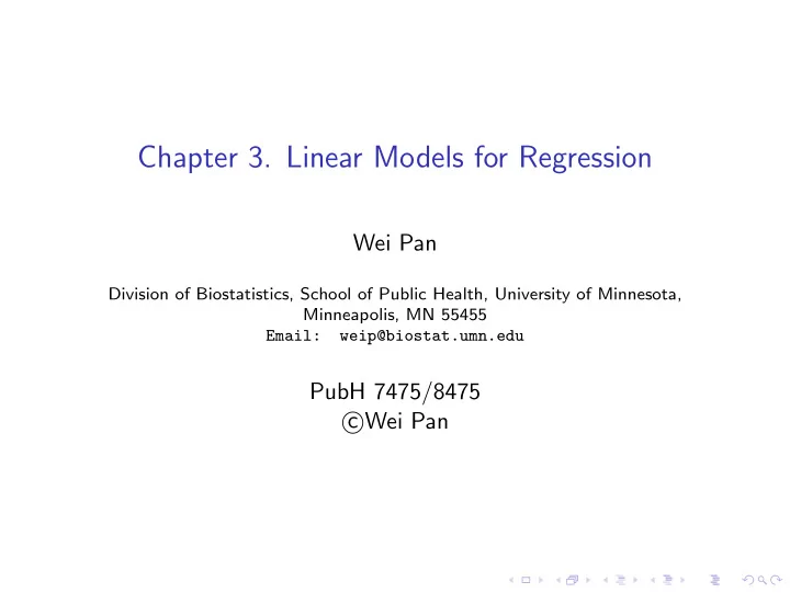
Chapter 3. Linear Models for Regression Wei Pan Division of Biostatistics, School of Public Health, University of Minnesota, Minneapolis, MN 55455 Email: weip@biostat.umn.edu PubH 7475/8475 � Wei Pan c

Linear Model and Least Squares ◮ Data: ( Y i , X i ), X i = ( X i 1 , ..., X ip ) ′ , i = 1 , ..., n . Y i : continuous ◮ LM: Y i = β 0 + � p j =1 X ij β j + ǫ i , ǫ i ’s iid with E ( ǫ i ) = 0 and Var ( ǫ i ) = σ 2 . j =1 X ij β j ) 2 = || Y − X β || 2 ◮ RSS ( β ) = � n i =1 ( Y i − β 0 − � p 2 . ◮ LSE (OLSE): ˆ β = arg min β RSS ( β ) = ( X ′ X ) − 1 X ′ Y . ◮ Nice properties: Under true model, E (ˆ β ) = β , Var (ˆ β ) = σ 2 ( X ′ X ) − 1 , β ∼ N ( β, Var (ˆ ˆ β )), Gauss-Markov Theorem: ˆ β has min var among all linear unbiased estimates.

◮ Some questions: σ 2 = RSS (ˆ ˆ β ) / ( n − p − 1). Q: what happens if the denominator is n ? Q: what happens if X ′ X is (nearly) singular? ◮ What if p is large relative to n ? ◮ Variable selection: forward, backward, stepwise: fast, but may miss good ones; best-subset: too time consuming.

Elements of Statistical Learning (2nd Ed.) � Hastie, Tibshirani & Friedman 2009 Chap 3 c Best Subset 0.95 Forward Stepwise Backward Stepwise β ( k ) − β || 2 Forward Stagewise 0.90 0.85 E || ˆ 0.80 0.75 0.70 0.65 0 5 10 15 20 25 30 Subset Size k FIGURE 3.6. Comparison of four subset-selection techniques on a simulated linear regression problem = X T β + ε . Y There are N = 300 observations on p = 31 standard Gaussian variables, with pair- wise correlations all equal to 0 . 85 . For 10 of the vari- ables, the coefficients are drawn at random from a N (0 , 0 . 4) distribution; the rest are zero. The noise

Shrinkage or regularization methods ◮ Use regularized or penalized RSS: PRSS ( β ) = RSS ( β ) + λ J ( β ) . λ : penalization parameter to be determined; (thinking about the p-value thresold in stepwise selection, or subset size in best-subset selection.) J (): prior; both a loose and a Bayesian interpretations; log prior density. ◮ Ridge: J ( β ) = � p j =1 β 2 j ; prior: β j ∼ N (0 , τ 2 ). β R = ( X ′ X + λ I ) − 1 X ′ Y . ˆ ◮ Properties: biased but small variances, E (ˆ β R ) = ( X ′ X + λ I ) − 1 X ′ X β , β R ) = σ 2 ( X ′ X + λ I ) − 1 X ′ X ( X ′ X + λ I ) − 1 ≤ Var (ˆ Var (ˆ β ), df ( λ ) = tr [ X ( X ′ X + λ I ) − 1 X ′ ] ≤ df (0) = tr ( X ( X ′ X ) − 1 X ′ ) = tr (( X ′ X ) − 1 X ′ X ) = p ,

◮ Lasso: J ( β ) = � p j =1 | β j | . Prior: β j Laplace or DE(0, τ 2 ); No closed form for ˆ β L . ◮ Properties: biased but small variances, df (ˆ β L ) = # of non-zero ˆ β L j ’s (Zou et al ). ◮ Special case: for X ′ X = I , or simple regression ( p = 1), ˆ j = ST(ˆ β j , λ ) = sign(ˆ β j )( | ˆ β L β j | − λ ) + , compared to: ˆ j = ˆ β R β j / (1 + λ ), ˆ j = HT(ˆ β j , M ) = ˆ β j I (rank(ˆ β B β j ) ≤ M ). ◮ A key property of Lasso: ˆ j = 0 for large λ , but not ˆ β L β R j . –simultaneous parameter estimation and selection.

◮ Note: for a convex J ( β ) (as for Lasso and Ridge), min PRSS is equivalent to: min RSS ( β ) s.t. J ( β ) ≤ t . ◮ Offer an intutive explanation on why we can have ˆ β L j = 0; see Fig 3.11. Theory: | β j | is singular at 0; Fan and Li (2001). ◮ How to choose λ ? obtain a solution path ˆ β ( λ ), then, as before, use tuning data or CV or model selection criterion (e.g. AIC or BIC). ◮ Example: R code ex3.1.r

Elements of Statistical Learning (2nd Ed.) � Hastie, Tibshirani & Friedman 2009 Chap 3 c β β 2 . . ^ ^ 2 β β β β 1 1 FIGURE 3.11. Estimation picture for the lasso (left) and ridge regression (right). Shown are contours of the error and constraint functions. The solid blue areas are the constraint regions | β 1 | + | β 2 | ≤ t and β 2 1 + β 2 2 ≤ t 2 , respectively, while the red ellipses are the contours of the least squares error function.

Elements of Statistical Learning (2nd Ed.) � Hastie, Tibshirani & Friedman 2009 Chap 3 c • lcavol • • • 0.6 • • • • • • • 0.4 • • • svi • • • • • • lweight • • • • • • • • • • • Coefficients • • • • pgg45 • • • • • • • • • • • • • • 0.2 • • • lbph • • • • • • • • • • • • • • • • • • • • • • • • • • • • • • • • • • • • • • • • • • • • • • • • • • • • • • • • • • • • • • • • • • • • • • • • • • • • • • • • • • • • • • • • • • • • • • • • • • • • • • • • • • • • • • 0.0 • • • • • • • • • • • • • • • • • gleason • • • • • • • • • • • • • • • • • age • −0.2 • • • lcp 0 2 4 6 8 df( λ )

Elements of Statistical Learning (2nd Ed.) � Hastie, Tibshirani & Friedman 2009 Chap 3 c lcavol 0.6 0.4 svi lweight pgg45 Coefficients lbph 0.2 0.0 gleason age −0.2 lcp 0.0 0.2 0.4 0.6 0.8 1.0 Shrinkage Factor s

◮ Lasso: biased estimates; alternatives: ◮ Relaxed lasso: 1) use Lasso for VS; 2) then use LSE or MLE on the selected model. ◮ Use a non-convex penalty: later... SCAD: eq (3.82) on p.92; j | β j | q with 0 < q < 1; Bridge J ( β ) = � j | β j | / | ˜ Adaptive Lasso (Zou 2006): J ( β ) = � β j , 0 | ; Truncated Lasso Penalty (Shen, Pan &Zhu 2012, JASA): J ( β ; τ ) = � j min( | β j | , τ ), or J ( β ; τ ) = � j min( | β j | /τ, 1). ◮ Choice b/w Lasso and Ridge: bet on a sparse model? risk prediction for GWAS (Austin, Pan & Shen 2013, SADM ). ◮ Elastic net (Zou & Hastie 2005): � α | β j | + (1 − α ) β 2 J ( β ) = j j may select more (correlated) X j ’s.

R packages for penalized GLMs (and Cox PHM) ◮ glmnet : Ridge, Lasso and Elastic net. ◮ ncvregi : SCAD, MCP. ◮ glmtlp : TLP. ◮ FGSG : grouping/fusion penalties (based on Lasso, TLP, etc) for LMs ◮ More general convex programming: Matlab CVX package.

(8000) Computational Algorithms for Lasso ◮ Quadratic programming: the original; slow. ◮ LARS ( § 3.8): the solution path is piece-wise linear; at a cost of fitting a single LM; not general? ◮ Incremental Forward Stagewise Regression ( § 3.8): approx; related to boosting. β ( r ) j / | ˆ ◮ A simple (and general) way: | β j | = β 2 | ; j truncate a current estimate | ˆ β ( r ) | ≈ 0 at a small ǫ . j ◮ Coordinate-descent algorithm ( § 3.8.6): update each β j while fixing others at the current estimates–recall we have a closed-form solution for a single β j ! simple and general but not applicable to grouping penalties. ◮ ADMM (Boyd et al 2011). http://stanford.edu/~boyd/admm.html

Sure Independence Screening (SIS) ◮ Q: penalized (or stepwise ...) regression can do automatic VS; just do it? ◮ Key: there is a cost/limit in performance/speed/theory. ◮ Q2: some methods (e.g. LDA/QDA/RDA) do not have VS, then what? ◮ Going back to basics: first conduct VS in marginal analysis, 1) Y ∼ X 1 , Y ∼ X 2 , ..., Y ∼ X p ; 2) choose a few top ones, say p 1 ; p 1 can be chosen somewhat arbitrarily, or treated as a tuning parameter 3) then apply penalized reg (or other VS) to the selected p 1 variables. ◮ Called SIS with theory (Fan & Lv, 2008, JRSS-B). R package SIS ; iterative SIS (ISIS); why? a limitation of SIS ...

Using Derived Input Directions ◮ PCR: PCA on X , then use the first few PCs as predictors. Use a few top PCs explaining a majority (e.g. 85% or 95%) of total variance; # of components: a tuning parameter; use (genuine) CV; Used in genetic association studies, even for p < n to improve power. +: simple; -: PCs may not be related to Y .

◮ Partial least squares (PLS): multiple versions; see Alg 3.3. Main idea: 1) regress Y on each X j univariately to obtain coef est φ 1 j ; 2) first component is Z 1 = � j φ 1 j X j ; 3) regress X j on Z 1 and use the residuals as new X j ; 4) repeat the above process to obtain Z 2 , ...; 5) Regress Y on Z 1 , Z 2 , ... ◮ Choice of # components: tuning data or CV (or AIC/BIC?) ◮ Contrast PCR and PLS: PCA: max α Var( X α ) s.t. ....; PLS: max α Cov( Y , X α ) s.t. ...; Continuum regression (Stone & Brooks 1990, JRSS-B) ◮ Penalized PCA (...) and Penalized PLS (Huang et al 2004, BI; Chun & Keles 2012, JRSS-B; R packages ppls, spls). ◮ Example code: ex3.2.r