bijgevoegde stelling Temporal dependencies for natural events - PowerPoint PPT Presentation

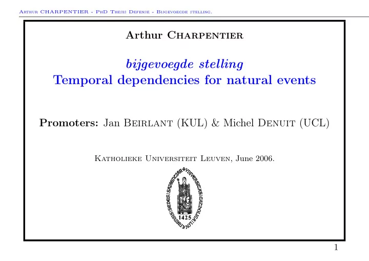
Arthur CHARPENTIER - PhD Thesis Defense - Bijgevoegde stelling. Arthur Charpentier bijgevoegde stelling Temporal dependencies for natural events Promoters: Jan Beirlant (KUL) & Michel Denuit (UCL) Katholieke Universiteit Leuven , June 2006. 1

Arthur CHARPENTIER - PhD Thesis Defense - Bijgevoegde stelling. Modeling daily windspeed and temperature Consider some stationary time series ( X t ) t ∈ Z , and define γ X ( h ) = cov ( X t , X t − h ) and its Fourier transform f X ( ω ) = 1 � γ X ( h ) cos( ωh ) . 2 π h ∈ Z Define autocorrelations as ρ X ( h ) = γ X ( h ) /γ X (0) . Long rang dependence: � h ∈ Z | ρ X ( h ) | = ∞ . Haslett & Rasftery (1989), ARFIMA processes for windspeed (1 − L ) d Φ( L ) X t = Θ( L ) ε t , where d ∈ (0 , 1) . GARMA processes, Hosking (1981, 1984), (1 − 2 uL + L 2 ) − λ Φ( L ) X t = Θ( L ) ε t , where λ ∈ (0 , 1 / 2) , | u | < 1 . ω = cos − 1 ( u ) is related to the seasonality of the series (e.g. ω = 2 π/ 365 ). σ 2 = 4 . 47 2 . For daily windpspeed ˆ λ = 0 . 126 and ˆ 2

Arthur CHARPENTIER - PhD Thesis Defense - Bijgevoegde stelling. 1.0 1.0 0.8 0.8 0.6 0.6 ACF ACF 0.4 0.4 0.2 0.2 0.0 0.0 0 20 40 60 80 100 0 500 1000 1500 2000 2500 3000 Lag Lag Figure 1: Autocorrelations, daily windspeed in Ireland. 3

Arthur CHARPENTIER - PhD Thesis Defense - Bijgevoegde stelling. Daily windspeed in Ireland 10 20 30 x$V1 0 1965 1970 1975 date Autocorrelation of daily time series 0.8 ACF 0.4 0.0 0 200 400 600 800 1000 Lag Series: x Smoothed Periodogram 200 spectrum 5 20 0.0 0.1 0.2 0.3 0.4 0.5 frequency bandwidth = 0.000434 Figure 2: Daily windspeed in Ireland. 4

Arthur CHARPENTIER - PhD Thesis Defense - Bijgevoegde stelling. 15 knots 20 knots 25 knots 2 days GARMA 47 . 7% 8 . 5% 0 . 3% seasonal ARMA 36 . 9% 3 . 6% 0 . 0% ratio 0 . 775 0 . 421 0 . 117 3 days GARMA 46 . 3% 8 . 0% 0 . 3% seasonal ARMA 27 . 7% 1 . 4% 0 . 0% ratio 0 . 597 0 . 176 0 . 010 4 days GARMA 45 . 3% 7 . 6% 0 . 3% seasonal ARMA 20 . 6% 0 . 5% 0 . 0% ratio 0 . 454 0 . 062 0 . 001 Table 1: Probabilities to have strong wind during consecutive days. 5

Arthur CHARPENTIER - PhD Thesis Defense - Bijgevoegde stelling. Minimal daily temperature in Paris (1997−2003) Maximal daily temperature in Paris (1997−2003) 220 300 200 250 Temperature in ’0.1 °C Temperature in ’0.1 °C 180 160 200 140 150 120 100 100 0 10 20 30 40 50 60 0 10 20 30 40 50 60 July and August July and August Figure 3: Daily temperature in Paris, years 1997 to 2003. 6

Arthur CHARPENTIER - PhD Thesis Defense - Bijgevoegde stelling. Daily minima in Paris − detrended (in °C) Daily Minimum Temperatures in Paris 10 0 x 20 −20 0 10000 20000 30000 15 Time Autocorrelation of daily time series 10 Temperature (°C) 0.5 5 ACF −0.5 0 0 200 400 600 800 1000 Lag −5 Series: x Smoothed Periodogram −10 spectrum 100 1 1900 1920 1940 1960 1980 2000 0.0 0.1 0.2 0.3 0.4 0.5 date frequency bandwidth = 7.63e−05 Figure 4: Trend of the series, and analysis of the series of residuals. 7

Arthur CHARPENTIER - PhD Thesis Defense - Bijgevoegde stelling. Daily minima in Paris − detrended (in °C) 10 x.des 0 −15 0 10000 20000 30000 Time Autocorrelation of residuals 0.8 ACF 0.4 0.0 0 20 40 60 80 100 Lag Series: x Smoothed Periodogram spectrum 20.0 0.5 0.0 0.1 0.2 0.3 0.4 0.5 frequency bandwidth = 7.63e−05 Figure 5: Residuals ( ε t ) t ∈ Z . 8

Arthur CHARPENTIER - PhD Thesis Defense - Bijgevoegde stelling. QQ plot of residuals (Gaussian) QQ plot of residuals (Student) 10 10 5 5 Sample Quantiles Sample quantiles 0 0 −5 −5 −10 −10 −15 −15 −4 −2 0 2 4 −4 −2 0 2 4 Theoretical Quantiles Theoritical Quantiles Figure 6: Residuals ( ε t ) t ∈ Z , versus Gaussian and t -distribution. 9

Arthur CHARPENTIER - PhD Thesis Defense - Bijgevoegde stelling. Distribution function of the period of return Distribution function of the period of return 1.0 1.0 11 consecutive days exceeding 19 degrees 4 consecutive days exceeding 24 degrees 0.8 0.8 0.6 0.6 0.4 0.4 0.2 0.2 GARMA + Gaussian noise GARMA + Gaussian noise ARMA + t noise ARMA + t noise 0.0 0.0 ARMA + Gaussian noise ARMA + Gaussian noise 0 50 100 150 200 0 50 100 150 200 Years before next heat wave Years before next heat wave Density of the period of return Density of the period of return GARMA + Gaussian noise GARMA + Gaussian noise 0.030 ARMA + t noise ARMA + t noise 0.030 ARMA + Gaussian noise ARMA + Gaussian noise 11 consecutive days exceeding 19 degrees 4 consecutive days exceeding 24 degrees 0.025 0.025 0.020 0.020 0.015 0.015 0.010 0.010 0.005 0.005 0.000 0.000 0 50 100 150 200 0 50 100 150 200 Years before next heat wave Years before next heat wave Figure 7: Survival distributions and densities of time before the next heat wave event (optimistic scenario). 10

Arthur CHARPENTIER - PhD Thesis Defense - Bijgevoegde stelling. Distribution function of the period of return Distribution function of the period of return 1.0 1.0 11 consecutive days exceeding 19 degrees 4 consecutive days exceeding 24 degrees 0.8 0.8 0.6 0.6 0.4 0.4 0.2 0.2 GARMA + Gaussian noise GARMA + Gaussian noise ARMA + t noise ARMA + t noise 0.0 0.0 ARMA + Gaussian noise ARMA + Gaussian noise 0 50 100 150 200 0 50 100 150 200 Years before next heat wave Years before next heat wave Density of the period of return Density of the period of return GARMA + Gaussian noise GARMA + Gaussian noise 0.030 0.030 ARMA + t noise ARMA + t noise ARMA + Gaussian noise ARMA + Gaussian noise 11 consecutive days exceeding 19 degrees 4 consecutive days exceeding 24 degrees 0.025 0.025 0.020 0.020 0.015 0.015 0.010 0.010 0.005 0.005 0.000 0.000 0 50 100 150 200 0 50 100 150 200 Years before next heat wave Years before next heat wave Figure 8: Survival distributions and densities of time before the next heat wave event (pessimistic scenario). 11

Arthur CHARPENTIER - PhD Thesis Defense - Bijgevoegde stelling. • heat wave, type (A): 11 consecutive days with temperature exceeding 19 ◦ C, short memory short memory long memory short tail noise heavy tail noise short tail noise optimistic 88 years 69 years 53 years pessimistic 79 years 54 years 37 years Table 2: Periods of return (expected value, in years) before the next heat wave similar with August 2003 (type (A)). 12

Arthur CHARPENTIER - PhD Thesis Defense - Bijgevoegde stelling. • heat wave, type (B): 3 consecutive days with temperature exceeding 24 ◦ C, short memory short memory long memory short tail noise heavy tail noise short tail noise optimistic 115 years 59 years 76 years pessimistic 102 years 51 years 64 years Table 3: Periods of return (expected value, in years) before the next heat wave similar with August 2003 (type (B)). 13

Arthur CHARPENTIER - PhD Thesis Defense - Bijgevoegde stelling. Modeling flood events Two classical approaches, based on annualized maxima, • Hurst (1951), long memory Gaussian process • Gumbel (1958), i.i.d. observations Gumbel distributed Based on 100 years of observations, not enough to assess if observations are, or not, independent: impact on return periods. Another idea, Todorovic & Zelenhasic (1970) and Todorovic & Rousselle : consider flood event as a marked Poisson process. Financial ACD (Autoregressive Conditional Duration) approach of Engle & Russell (1998). 14

Arthur CHARPENTIER - PhD Thesis Defense - Bijgevoegde stelling. 600 observations 87 observations 1.0 1.0 0.8 0.8 0.6 0.6 autocorrelation autocorrelation 0.4 0.4 0.2 0.2 0.0 0.0 −0.2 0 5 10 15 20 25 0 5 10 15 lag lag Figure 9: Autocorrelation function of the Nile annual maxima series. 15

Arthur CHARPENTIER - PhD Thesis Defense - Bijgevoegde stelling. Let X i denote observed durations ( X i = T i − T i − 1 ), and define H i = σ ( X 1 , ...., X i − 1 ) . Assume that  X i = Ψ i · ε i , where ( ε i ) i.i.d. (Exponential or Weibull)    E ( X i |H i ) = Ψ i  Ψ i = ω + � p k =1 α k X i − k + � q  k =1 β k Ψ i − k ,  i.e. max { p,q } q � � X i = ω + ( α k + β k ) − β k η i − k + η i , k =1 k =1 where η i = X i − Ψ i = X i − E ( X i |H i − 1 ) . Two duration model in Engle & Lunde (2003): time between two flood events, and duration of the flood. Marked process, with peak of the flood and volume. Distribution of residuals ( ε i ) : exponential in finance, mixed Weibull in hydrology. 16

Arthur CHARPENTIER - PhD Thesis Defense - Bijgevoegde stelling. Figure 10: Two durations model 17

Arthur CHARPENTIER - PhD Thesis Defense - Bijgevoegde stelling. Theoretical vs. observed volume 10000 8000 Empirical observed volume 6000 4000 2000 0 0 1000 2000 3000 4000 5000 6000 7000 Theoretical volume Figure 11: Relationship between peak, volume and duration of a flood. 18

Arthur CHARPENTIER - PhD Thesis Defense - Bijgevoegde stelling. density(x = ttt) 0.6 0.5 0.4 Density 0.3 0.2 0.1 0.0 0 1 2 3 4 5 6 7 N = 243 Bandwidth = 0.3112 Figure 12: Kernel density estimation of residuals 19

Arthur CHARPENTIER - PhD Thesis Defense - Bijgevoegde stelling. 1.0 0.8 0.6 donnees 0.4 0.2 0.0 0.0 0.2 0.4 0.6 0.8 1.0 simulation Figure 13: Empirical distribution function of the data vs. Weibull mixture. 20