Approximation Algorithms Q. Suppose I need to solve an NP-hard - PowerPoint PPT Presentation

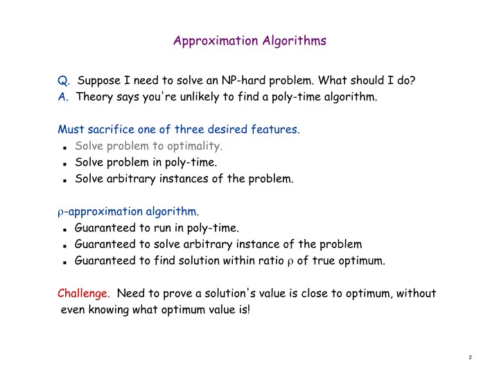
Approximation Algorithms Q. Suppose I need to solve an NP-hard problem. What should I do? A. Theory says you're unlikely to find a poly-time algorithm. Must sacrifice one of three desired features.  Solve problem to optimality.  Solve problem in poly-time.  Solve arbitrary instances of the problem. ρ -approximation algorithm.  Guaranteed to run in poly-time.  Guaranteed to solve arbitrary instance of the problem  Guaranteed to find solution within ratio ρ of true optimum. Challenge. Need to prove a solution's value is close to optimum, without even knowing what optimum value is! 2

11.1 Load Balancing

Load Balancing Input. m identical machines; n jobs, job j has processing time t j .  Job j must run contiguously on one machine.  A machine can process at most one job at a time. Def. Let J(i) be the subset of jobs assigned to machine i. The load of machine i is L i = Σ j ∈ J(i) t j . Def. The makespan is the maximum load on any machine L = max i L i . Load balancing. Assign each job to a machine to minimize makespan. 4

Load Balancing: List Scheduling List-scheduling algorithm.  Consider n jobs in some fixed order.  Assign job j to machine whose load is smallest so far. List-Scheduling(m, n, t 1 ,t 2 ,…,t n ) { for i = 1 to m { load on machine i L i ← 0 jobs assigned to machine i J(i) ← φ } for j = 1 to n { machine i has smallest load i = argmin k L k assign job j to machine i J(i) ← J(i) ∪ {j} L i ← L i + t j update load of machine i } } Implementation. O(n log n) using a priority queue. 5

Load Balancing: List Scheduling Analysis Theorem. [Graham, 1966] Greedy algorithm is a 2-approximation.  First worst-case analysis of an approximation algorithm.  Need to compare resulting solution with optimal makespan L*. Lemma 1. The optimal makespan L* ≥ max j t j . Pf. Some machine must process the most time-consuming job. ▪ Lemma 2. The optimal makespan 1 L * ≥ t j . ∑ j m Pf.  The total processing time is Σ j t j .  One of m machines must do at least a 1/m fraction of total work. ▪ 6

Load Balancing: List Scheduling Analysis Theorem. Greedy algorithm is a 2-approximation. Pf. Consider load L i of bottleneck machine i.  Let j be last job scheduled on machine i.  When job j assigned to machine i, i had smallest load. Its load before assignment is L i - t j ⇒ L i - t j ≤ L k for all 1 ≤ k ≤ m. blue jobs scheduled before j machine i j 0 L i - t j L = L i 7

Load Balancing: List Scheduling Analysis Theorem. Greedy algorithm is a 2-approximation. Pf. Consider load L i of bottleneck machine i.  Let j be last job scheduled on machine i.  When job j assigned to machine i, i had smallest load. Its load before assignment is L i - t j ⇒ L i - t j ≤ L k for all 1 ≤ k ≤ m.  Sum inequalities over all k and divide by m: L i − t j 1 L k ≤ ∑ m k 1 t k = ∑ m k Lemma 1 L * ≤  Now ▪ L i = ( L i − t j ) 4 + t j { ≤ 2 L *. 1 2 4 3 ≤ L * ≤ L * Lemma 2 8

Load Balancing: List Scheduling Analysis Q. Is our analysis tight? A. Essentially yes. Ex: m machines, m(m-1) jobs length 1 jobs, one job of length m machine 2 idle machine 3 idle machine 4 idle m = 10 machine 5 idle machine 6 idle machine 7 idle machine 8 idle machine 9 idle machine 10 idle list scheduling makespan = 19 9

Load Balancing: List Scheduling Analysis Q. Is our analysis tight? A. Essentially yes. Ex: m machines, m(m-1) jobs length 1 jobs, one job of length m m = 10 optimal makespan = 10 10

Load Balancing: LPT Rule Longest processing time (LPT). Sort n jobs in descending order of processing time, and then run list scheduling algorithm. LPT-List-Scheduling(m, n, t 1 ,t 2 ,…,t n ) { Sort jobs so that t 1 ≥ t 2 ≥ … ≥ t n for i = 1 to m { load on machine i L i ← 0 jobs assigned to machine i J(i) ← φ } for j = 1 to n { machine i has smallest load i = argmin k L k assign job j to machine i J(i) ← J(i) ∪ {j} L i ← L i + t j update load of machine i } } 11

Load Balancing: LPT Rule Observation. If at most m jobs, then list-scheduling is optimal. Pf. Each job put on its own machine. ▪ Lemma 3. If there are more than m jobs, L* ≥ 2 t m+1 . Pf.  Consider first m+1 jobs t 1 , …, t m+1 .  Since the t i 's are in descending order, each takes at least t m+1 time.  There are m+1 jobs and m machines, so by pigeonhole principle, at least one machine gets two jobs. ▪ Theorem. LPT rule is a 3/2 approximation algorithm. Pf. Same basic approach as for list scheduling. L i = ( L i − t j ) { ≤ 3 t j 2 L *. ▪ 4 + 1 2 4 3 ≤ 1 2 L * ≤ L * Lemma 3 ( by observation, can assume number of jobs > m ) 12

Load Balancing: LPT Rule Q. Is our 3/2 analysis tight? A. No. Theorem. [Graham, 1969] LPT rule is a 4/3-approximation. Pf. More sophisticated analysis of same algorithm. Q. Is Graham's 4/3 analysis tight? A. Essentially yes. Ex: m machines, n = 2m+1 jobs, 2 jobs of length m+1, m+2, …, 2m-1 and one job of length m. 13

11.2 Center Selection

Center Selection Problem Input. Set of n sites s 1 , …, s n . Center selection problem. Select k centers C so that maximum distance from a site to nearest center is minimized. k = 4 r(C) center site 15

Center Selection Problem Input. Set of n sites s 1 , …, s n . Center selection problem. Select k centers C so that maximum distance from a site to nearest center is minimized. Notation.  dist(x, y) = distance between x and y.  dist(s i , C) = min c ∈ C dist(s i , c) = distance from s i to closest center.  r(C) = max i dist(s i , C) = smallest covering radius. Goal. Find set of centers C that minimizes r(C), subject to |C| = k. Distance function properties.  dist(x, x) = 0 (identity)  dist(x, y) = dist(y, x) (symmetry)  dist(x, y) ≤ dist(x, z) + dist(z, y) (triangle inequality) 16

Center Selection Example Ex: each site is a point in the plane, a center can be any point in the plane, dist(x, y) = Euclidean distance. Remark: search can be infinite! r(C) center site 17

Greedy Algorithm: A False Start Greedy algorithm. Put the first center at the best possible location for a single center, and then keep adding centers so as to reduce the covering radius each time by as much as possible. Remark: arbitrarily bad! greedy center 1 center k = 2 centers site 18

Center Selection: Greedy Algorithm Greedy algorithm. Repeatedly choose the next center to be the site farthest from any existing center. Greedy-Center-Selection(k, n, s 1 ,s 2 ,…,s n ) { C = φ repeat k times { Select a site s i with maximum dist(s i , C) Add s i to C site farthest from any center } return C } Observation. Upon termination all centers in C are pairwise at least r(C) apart. Pf. By construction of algorithm. 19

Center Selection: Analysis of Greedy Algorithm Theorem. Let C* be an optimal set of centers. Then r(C) ≤ 2r(C*). Pf. (by contradiction) Assume r(C*) < ½ r(C).  For each site c i in C, consider ball of radius ½ r(C) around it.  Exactly one c i * in each ball; let c i be the site paired with c i *.  Consider any site s and its closest center c i * in C*.  dist(s, C) ≤ dist(s, c i ) ≤ dist(s, c i *) + dist(c i *, c i ) ≤ 2r(C*).  Thus r(C) ≤ 2r(C*). ▪ Δ -inequality ≤ r(C*) since c i * is closest center ½ r(C) ½ r(C) c i ½ r(C) C* c i * sites s 20

Center Selection Theorem. Let C* be an optimal set of centers. Then r(C) ≤ 2r(C*). Theorem. Greedy algorithm is a 2-approximation for center selection problem. Remark. Greedy algorithm always places centers at sites, but is still within a factor of 2 of best solution that is allowed to place centers anywhere. e.g., points in the plane Question. Is there hope of a 3/2-approximation? 4/3? Theorem. Unless P = NP, there no ρ -approximation for center-selection problem for any ρ < 2. 21