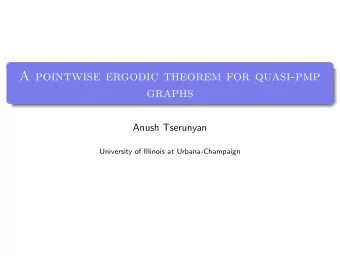
A pointwise ergodic theorem for imprecise Markov chains Gert de - PowerPoint PPT Presentation

A pointwise ergodic theorem for imprecise Markov chains Gert de Cooman Jasper De Bock Stavros Lopatatzidis Ghent University, SYSTeMS {gert.decooman,jasper.debock,stavros,lopatatzidis}@UGent.be http://users.UGent.be/˜gdcooma gertekoo.wordpress.com ISIPTA 2015 Pescara, 23 July 2015

My boon companions JASPER DE BOCK STAVROS LOPATATZIDIS

A discrete-time finite-state uncertain process Uncertain variables X 1 , X 2 , . . . , X n , . . . assuming values in some finite set of states X .

A simple discrete-time finite-state uncertain process ( b , b , b ) ( b , b ) ( b , b , a ) b ( b , a , b ) ( b , a ) ( b , a , a ) ( a , b , b ) ( a , b ) ( a , b , a ) a ( a , a , b ) ( a , a ) ( a , a , a )

A simple discrete-time finite-state uncertain process ( b , b , b ) ( b , b ) situations ( b , b , a ) set of paths ω = sample space Ω b ( b , a , b ) ( b , a ) ( b , a , a ) ( a , b , b ) ( a , b ) ( a , b , a ) a ( a , a , b ) ( a , a ) ( a , a , a )

A simple discrete-time finite-state uncertain process ( b , b , b ) ( b , b ) q ( ·| b , b ) ( b , b , a ) q ( ·| b ) b ( b , a , b ) ( b , a ) q ( ·| b , a ) ( b , a , a ) q ( ·| � ) ( a , b , b ) ( a , b ) q ( ·| a , b ) ( a , b , a ) q ( ·| a ) a ( a , a , b ) ( a , a ) q ( ·| a , a ) ( a , a , a )

A simple discrete-time finite-state uncertain process ( b , b , b ) Q ( ·| b , b ) ( b , b ) ( b , b , a ) Q ( ·| b ) b ( b , a , b ) ( b , a ) Q ( ·| b , a ) ( b , a , a ) Q ( ·| � ) ( a , b , b ) Q ( ·| a , b ) ( a , b ) ( a , b , a ) Q ( ·| a ) a ( a , a , b ) ( a , a ) Q ( ·| a , a ) ( a , a , a )

An event tree and its situations and paths Situations are nodes in the event tree. situation s = ( x 1 , x 2 ,..., x n ) = x 1: n The sample space Ω is the set of all paths. path ω = ( x 1 , x 2 ,..., x n ,... ) ∈ X N An event A is a subset of the sample space Ω : A ⊆ Ω .

Processes and process differences A real process F is a real function defined on situations: F ( s , a ) = − 5 s , a s , b F ( s , b ) = − 3 F ( s ) = 2 F ( s , c ) = 0 s , c s F ( s , d ) = 9 s , d F ( s , e ) = − 5 s , e D ( s ) and its process difference: ∆ F ( s ) = F ( s · ) − F ( s ) ∈ G ( D ( s )) for all situations s

Sub- and supermartingales We can use the local models Q ( ·| s ) to define sub- and supermartingales: A submartingale M is a real process such that in all non-terminal situations s : Q ( ∆ M ( s ) | s ) ≥ 0 . A supermartingale M is a real process such that in all non-terminal situations s : Q ( ∆ M ( s ) | s ) ≤ 0 .

Lower and upper expectations The most conservative coherent lower and upper expectations on G ( Ω ) that coincide with the local models and satisfy a number of additional continuity criteria (cut conglomerability and cut continuity): Conditional lower expectations: � � E ( f | s ) : = sup M ( s ) : limsup M ( s • ) ≤ f ( s • ) Conditional upper expectations: � � E ( f | s ) : = inf M ( s ) : liminf M ( s • ) ≥ f ( s • )

Test supermartingales and strictly null events A test supermartingale T is a non-negative supermartingale with T ( � ) = 1 . (Very close to Ville’s definition of a martingale.) An event A is strictly null if there is some test supermartingale T that converges to + ∞ on A : n → ∞ T ( ω n ) = + ∞ for all ω ∈ A . lim T ( ω ) = lim If A is strictly null then � � P ( A ) = E ( I A ) = inf M ( � ) : liminf M ≥ I A = 0 .

SLLN for submartingale differences (De Cooman and De Bock, 2013) Consider any submartingale M such that its difference process ∆ M ( s ) = M ( s · ) − M ( s ) ∈ G ( D ( s )) for all non-terminal s is uniformly bounded. Then liminf � M � ≥ 0 strictly almost surely, or in other words n 1 1 ∑ � � ∆ M ( X 1 ,..., X k − 1 )( X k ) = liminf M ( X 1 ,... X n ) − M ( � ) ≥ 0 liminf n n n → + ∞ n → + ∞ k = 1 In particular, for any real function f on X : n 1 ∑ � � f ( X k ) − Q ( f ( X k | X 1: k − 1 ) ≥ 0 strictly almost surely liminf n n → + ∞ k = 1

SLLN for submartingale differences (De Cooman and De Bock, 2013) Consider any submartingale M such that its difference process ∆ M ( s ) = M ( s · ) − M ( s ) ∈ G ( D ( s )) for all non-terminal s is uniformly bounded. Then liminf � M � ≥ 0 strictly almost surely, or in other words n 1 1 ∑ � � ∆ M ( X 1 ,..., X k − 1 )( X k ) = liminf M ( X 1 ,... X n ) − M ( � ) ≥ 0 liminf n n n → + ∞ n → + ∞ k = 1 In particular, for any real function f on X : n 1 ∑ f ( X k ) ≥ Q ( f ) strictly almost surely liminf n n → + ∞ k = 1

Imprecise Markov chains

@ARTICLE{cooman2009, author = {{d}e Cooman, Gert and Hermans, Filip and Quaegehebeur, Erik}, title = {Imprecise {M}arkov chains and their limit behaviour}, journal = {Probability in the Engineering and Informational Sciences}, year = 2009, volume = 23, pages = {597--635}, doi = {10.1017/S0269964809990039} }

A simple discrete-time finite-state stochastic process ( b , b , b ) Q ( ·| b , b ) ( b , b ) ( b , b , a ) Q ( ·| b ) b ( b , a , b ) ( b , a ) Q ( ·| b , a ) ( b , a , a ) Q ( ·| � ) ( a , b , b ) Q ( ·| a , b ) ( a , b ) ( a , b , a ) Q ( ·| a ) a ( a , a , b ) ( a , a ) Q ( ·| a , a ) ( a , a , a )

An imprecise IID model ( b , b , b ) Q ( ·| � ) ( b , b ) ( b , b , a ) Q ( ·| � ) b ( b , a , b ) ( b , a ) Q ( ·| � ) ( b , a , a ) Q ( ·| � ) ( a , b , b ) Q ( ·| � ) ( a , b ) ( a , b , a ) Q ( ·| � ) a ( a , a , b ) ( a , a ) Q ( ·| � ) ( a , a , a )

An imprecise Markov chain ( b , b , b ) Q ( ·| b ) ( b , b ) ( b , b , a ) Q ( ·| b ) b ( b , a , b ) ( b , a ) Q ( ·| a ) ( b , a , a ) Q ( ·| � ) ( a , b , b ) Q ( ·| b ) ( a , b ) ( a , b , a ) Q ( ·| a ) a ( a , a , b ) ( a , a ) Q ( ·| a ) ( a , a , a )

Stationarity and ergodicity The lower expectation E n for the state X n at time n : E n ( f ) = E ( f ( X n )) The imprecise Markov chain is Perron–Frobenius-like if for all marginal models E 1 and all f : E n ( f ) → E ∞ ( f ) . and if E 1 = E ∞ then E n = E ∞ , and the imprecise Markov chain is stationary. In any Perron–Frobenius-like imprecise Markov chain: n 1 ∑ E n ( f ) = E ∞ ( f ) lim n → + ∞ n k = 1 and n n 1 1 ∑ ∑ E ∞ ( f ) ≤ liminf f ( X k ) ≤ limsup f ( X k ) ≤ E ∞ ( f ) str. almost surely . n n n → + ∞ n → + ∞ k = 1 k = 1

The essence of the argument From n 1 ∑ � � f ( X k ) − Q ( f ( X k ) | X k − 1 ) ≥ 0 strictly almost surely liminf n → + ∞ n k = 1 to n 1 ∑ � � liminf f ( X k ) − E ∞ ( f ) ≥ 0 strictly almost surely n → + ∞ n k = 1