A Localized Markov Chain Particle Filter (LMCPF) for the Global - PowerPoint PPT Presentation
A Localized Markov Chain Particle Filter (LMCPF) for the Global Weather Prediction Model ICON Anne Sophie Walter and Roland Potthast and Andreas Rhodin German Meteorological Service (DWD) Data Assimilation Unit 7th International Symposium on
A Localized Markov Chain Particle Filter (LMCPF) for the Global Weather Prediction Model ICON Anne Sophie Walter and Roland Potthast and Andreas Rhodin German Meteorological Service (DWD) Data Assimilation Unit 7th International Symposium on Data Assimilation 2019
What is new? • Two localized particle filters working stably in an operational setup: LAPF and LMCPF • Strong improvements of scores by including model error via a Gaussian mixture approach for the prior distribution • LMCPF partly decouples spread and assimilation functionality (via model error) • First particle filter tests with full global operational resolution and setup, including two-way European nest in global DA • Particle Filter shows behavior similar to LETKF, with some scores better than LETKF, some worse (o-b and forecast!) • LMCPF also works similarly for COSMO convective scale 22.01.2019 anne.walter@dwd.de 2 A Localized Markov Chain Particle Filter for the Global Weather Prediction Model ICON
Content 1. The ICON-Model and DA-System 2. The Localized Markov Chain Particle Filter (LMCPF) 3. Numerical Testing 4. Summary 22.01.2019 anne.walter@dwd.de 3 A Localized Markov Chain Particle Filter for the Global Weather Prediction Model ICON
1. The ICON-Model • Operational NWP model of DWD: ICON (ICOsahedral Nonhydrostatic) • Two-way NEST over Europe (~6.5 km) • Resolution: 13 km deterministic 40 km ensemble (40 member) 22.01.2019 anne.walter@dwd.de 4 A Localized Markov Chain Particle Filter for the Global Weather Prediction Model ICON
1. DA System at DWD • Hybrid EnVar operational since January 20, 2016 𝑌 𝑏 = ҧ 𝑦 𝑐 + 𝑌 𝑐 𝑋 • Following Hunt et al. (2007), B-Matrix (see also Schraff et al., 2016) • EnVar-B-Matrix: 70% LETKF, 30% Climatology 22.01.2019 anne.walter@dwd.de 5 A Localized Markov Chain Particle Filter for the Global Weather Prediction Model ICON
2. The LMCPF • Our Particle Filters are based on the LETKF philosophy ➢ Localization: as LETKF in ensemble space ➢ Adaptivity: tools for spread control PRIOR DATA ➢ Able to handle with multi-modal distributions ➢ Able to handle with Non-Gaussianity Posterior Analysis Ensemble 22.01.2019 anne.walter@dwd.de 6 A Localized Markov Chain Particle Filter for the Global Weather Prediction Model ICON
2. The LMCPF LETKF DATA Posterior Prior LMCPF Classical PF DATA DATA Prior Posterior Posterior Prior 22.01.2019 anne.walter@dwd.de 7 A Localized Markov Chain Particle Filter for the Global Weather Prediction Model ICON
2. The LMCPF First Step: The Classical Particle Filter • Employ Bayes formula to calculate new analysis distribution 𝑏 𝑦 : = 𝑞 𝑦 𝑧 𝑙 = 𝑑 𝑞 𝑧 𝑙 𝑦 𝑞 𝑙 𝑐 𝑦 , 𝑦 ∈ ℝ 𝑜 𝑞 𝑙 𝑏 𝑑 is a normalization factor: 𝑌 𝑞 𝑙 𝑦 𝑒𝑦 = 1 𝑏 are • To carry out the analysis step at time 𝑢 𝑙 a posteriori weights 𝑥 𝑙,𝑚 calculated (𝑏) = 𝑑 𝑓 −1 𝑈 𝑆 −1 (𝑧−𝐼𝑦 𝑚 ) 2 𝑧−𝐼𝑦 𝑚 𝑥 𝑙,𝑚 (𝑏) = 𝑀 𝑀 𝑑 is chosen such that σ 𝑚=1 𝑥 𝑙,𝑚 22.01.2019 anne.walter@dwd.de 8 A Localized Markov Chain Particle Filter for the Global Weather Prediction Model ICON
2. The LMCPF Second Step: Classical Resampling • Accumulated weights 𝑥 𝑏𝑑 are defined: 𝑥 𝑏𝑑 0 = 0 𝑏 , 𝑥 𝑏𝑑 𝑚 = 𝑥 𝑏𝑑 𝑚−1 + 𝑥 𝑚 𝑚 = 1, … , 𝑀 where 𝑀 denotes the ensemble size • Drawing 𝑠 𝑚 ~𝑉 0,1 , 𝑚 = 1, … , 𝑀 , set 𝑆 𝑚 = 𝑚 − 1 + 𝑠 𝑚 and define transform matrix ෲ 𝑿 for the particles by: 𝑗,𝑚 = ൝1 𝑗𝑔 𝑆 𝑚 ∈ 𝑥 𝑏𝑑 𝑚−1 , 𝑥 𝑏𝑑 𝑚 , ෲ 𝑋 0 𝑝𝑢ℎ𝑓𝑠𝑥𝑗𝑡𝑓, 𝑗, 𝑚 = 1, … , 𝑀 with 𝑋 ∈ ℝ 𝑀𝑦𝑀 , (𝑡, 𝑢] denotes the interval of values 𝑡 < 𝜃 ≤ 𝑢 . 22.01.2019 anne.walter@dwd.de 9 A Localized Markov Chain Particle Filter for the Global Weather Prediction Model ICON
2. The LMCPF Third Step: Spread Control • Based on the adaptive multiplicative inflation factor 𝝇 determined by the LETKF 𝑈 𝜍 = Ε 𝒆 𝑝−𝑐 𝒆 𝑝−𝑐 − Tr(𝐒) 𝑈𝑠(𝑰𝑸 𝑐 𝑰 𝑈 ) • Weighting factor 𝜷 has been chosen, due to the small ensemble size ( 𝑀 = 40 ) 𝜍 𝑙 = 𝛽 𝜍 𝑙 + 1 − 𝛽 𝜍 𝑙−1 22.01.2019 anne.walter@dwd.de 10 A Localized Markov Chain Particle Filter for the Global Weather Prediction Model ICON
2. The LMCPF Third Step: Spread Control • Perturbation factor 𝜏 is used to add spread to the system 𝜍 < 𝜍 (0) 𝑑 0 , 𝑑 0 + 𝑑 1 − 𝑑 0 ∗ 𝜍 − 𝜍 (0) 𝜍 (0) ≤ 𝜍 ≤ 𝜍 (1) 𝜏 = 𝜍 (1) − 𝜍 (0) , 𝜍 > 𝜍 (1) 𝑑 1 , where 𝑑 0 = 0.02 , 𝑑 1 = 1.5 , 𝜍 (0) = 1.0 and 𝜍 (1) = 1.4 , with 𝜏 = 𝑑 1 if 𝜍 ≥ 𝜍 (1) and 𝜏 = 𝑑 0 if 𝜍 ≤ 𝜍 (0) 22.01.2019 anne.walter@dwd.de 11 A Localized Markov Chain Particle Filter for the Global Weather Prediction Model ICON
2. The LMCPF Fourth Step: Determine posterior B ≡ ෨ 𝐶 ෨ 𝐿 = 𝐶𝐼 𝑈 𝑆 + 𝐼𝐶𝐼 𝑈 −1 𝐶 = 𝐽 − 𝐿𝐼 𝐶 = 𝐽 − 𝐶𝐼 𝑈 𝑆 + 𝐼𝐶𝐼 𝑈 −1 𝐼 𝐶 𝐶 = 𝛿𝑌𝑌 𝑈 = 𝐽 − 𝛿𝑌 𝑌 𝑈 𝐼 𝑈 𝑆 + 𝛿 𝐼𝑌 𝑌 𝑈 𝐼 𝑈 −1 𝐼 𝛿𝑌𝑌 𝑈 𝐼𝑌 = 𝑍 = 𝑌(𝐽 − 𝛿 𝑍 𝑈 (𝑆 + 𝛿𝑍𝑍 𝑈 ) −1 𝑍)𝛿𝑌 𝑈 𝑍 𝑈 𝑆 + 𝛿𝑍𝑍 𝑈 −1 = 𝐽 + 𝛿𝑍 𝑈 𝑆 −1 𝑍 −1 𝑍 𝑈 𝑆 −1 = 𝑌 𝐽 − 𝛿 𝐽 + 𝛿𝑍 𝑈 𝑆 −1 𝑍 −1 𝑍 𝑈 𝑆 −1 𝑍 𝛿X 𝑈 𝐽 + 𝛿𝑍 𝑈 𝑆 −1 𝑍 −1 (𝐽 + 𝛿𝑍 𝑈 𝑆 −1 𝑍 − 𝛿𝑍 𝑈 𝑆 −1 𝑍) 𝛿𝑌 𝑈 = 𝑌 = 𝑌 𝐽 + 𝛿𝑍 𝑈 𝑆 −1 𝑍 −1 𝛿𝑌 𝑈 = 𝛿𝑌 𝐽 + 𝛿𝑍 𝑈 𝑆 −1 𝑍 −1 𝑌 𝑈 22.01.2019 anne.walter@dwd.de 12 A Localized Markov Chain Particle Filter for the Global Weather Prediction Model ICON
2. The LMCPF Fifth Step: Calculation of the Shift-Vector 𝛾 (𝑡ℎ𝑗𝑔𝑢,𝑚) 𝛾 (𝑡ℎ𝑗𝑔𝑢,𝑚) = 𝐽 + 𝛿Y 𝑈 𝑆 −1 𝑍 −1 𝑍 𝑈 𝑆 −1 𝐷 − 𝑓 𝑚 with 𝐵 = 𝑍 𝑈 𝑆 −1 𝑍 , 𝐷 = 𝐵 −1 𝑍 𝑈 𝑆 −1 (𝑧 0 − ത 𝑧 𝑐 ) 𝑋 (𝑡ℎ𝑗𝑔𝑢) ≔ 𝛾 𝑡ℎ𝑗𝑔𝑢,1 , … , 𝛾 (𝑡ℎ𝑗𝑔𝑢,𝑀) ∈ ℝ 𝑀×𝑀 Important effects of 𝛾 (𝑡ℎ𝑗𝑔𝑢,𝑚) : • it moves the particles towards the observations in ensemble space • by the use of model error, it constitutes a further degree of freedom which can be used for tuning of a real system 22.01.2019 anne.walter@dwd.de 13 A Localized Markov Chain Particle Filter for the Global Weather Prediction Model ICON
2. The LMCPF Sixth Step: Gaussian Resampling • Weights W are calculated by drawing from the posterior 𝑋 + 𝑋 (𝑡ℎ𝑗𝑔𝑢) ∗ . 𝑋 = 𝑋 + ෨ 𝐶 ∗ 𝑆 𝑜𝑒 ∗ 𝜏 Centers of posterior RBFs Shape of posterior RBFs DATA with 𝑆 𝑜𝑒 normally distributed random numbers, 𝑋 (𝑡ℎ𝑗𝑔𝑢) and ෨ 𝐶 calculated with Gaussian radial basis function (rbf) Approximation for prior density and observation error Posterior Prior ➢ It is an explicit calculation of the Bayes posterior based on radial basis function approximation of the prior. 22.01.2019 anne.walter@dwd.de 14 A Localized Markov Chain Particle Filter for the Global Weather Prediction Model ICON
3. Numerical Testing
3. Numerical Testing Experimental setup (A) Experimental setup (B) • • Full ensemble: 40 members Full ensemble: 40 members • • Routine resolution: Reduced resolution: • 26km deterministic • 13km deterministic • 52km ensemble • 40km ensemble ➢ two-way NEST: • Period: 06.05.2016 – 31.05.2016 • 6.5km deterministic • 20km ensemble • Period: 01.09.2018 – 04.09.2018 • Lot more satellite data: SEVIRI, IASI & ATMS humidity channels T [K] at 03.05.2016 15 UTC ~1000 hPa 22.01.2019 anne.walter@dwd.de 16 A Localized Markov Chain Particle Filter for the Global Weather Prediction Model ICON
3. Numerical Testing Assimilation Cycle Experimental setup (A)
3. Numerical Testing – (A) Global RMSE for obs-fg statistics (Radiosondes vs. Model) Period: 10.05.2016 – 31.05.2016 Temperature Relative humidity ~7% p-level [hPa] LETKF LMCPF ~3% ~4% ~2% better RMSE RMSE 22.01.2019 anne.walter@dwd.de 18 A Localized Markov Chain Particle Filter for the Global Weather Prediction Model ICON
3. Numerical Testing – (A) Global RMSE for obs-fg statistics Period: 10.05.2016 – 31.05.2016 𝑈 𝐶𝑠𝑗ℎ𝑢𝑜𝑓𝑡𝑡 (IASI) Bending Angles (GPSRO) ~3% Channel number Height [m] LETKF LMCPF ~6% ~15% ~17% RMSE RMSE 22.01.2019 anne.walter@dwd.de 19 A Localized Markov Chain Particle Filter for the Global Weather Prediction Model ICON
3. Numerical Testing Assimilation Cycle Experimental setup (B)
3. Numerical Testing – (B) Global RMSE for obs-fg statistics (Radiosondes vs. Model) Period: 01.09.2018 – 04.09.2018 Temperature Relative humidity ~3% better ~2% p-level [hPa] LETKF LMCPF ~3% RMSE RMSE 22.01.2019 anne.walter@dwd.de 21 A Localized Markov Chain Particle Filter for the Global Weather Prediction Model ICON
Recommend
More recommend
Explore More Topics
Stay informed with curated content and fresh updates.
