A General Framework for Learning an Ensemble of Decision Rules - PowerPoint PPT Presentation

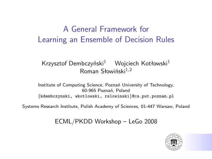
A General Framework for Learning an Ensemble of Decision Rules Krzysztof Dembczyński 1 Wojciech Kotłowski 1 Roman Słowiński 1 , 2 Institute of Computing Science, Poznań University of Technology, 60-965 Poznań, Poland { kdembczynski, wkotlowski, rslowinski } @cs.put.poznan.pl Systems Research Institute, Polish Academy of Sciences, 01-447 Warsaw, Poland ECML/PKDD Workshop – LeGo 2008

Motivation • Decision rule is a simple logical pattern in the form: ”if condition then decision ”. • A simple classifier voting for some class when the condition is satisfied and abstaining from vote otherwise. • Example: if duration > = 36 and savings status ≥ 1000 and employment � = unemployed and purpose = furniture/equipment , then risk level is low • Main advantage of decision rules is their simplicity and human-interpretable form handling interactions between attributes.

Motivation • The most popular rule induction algorithms are based on sequential covering : AQ, CN2, Ripper. • Forward stagewise additive modeling or boosting that treats rules as base classifiers in the ensemble can be seen as a generalization of sequential covering. • Algorithms such as RuleFit, SLIPPER, LRI or MLRules follow boosting approach and are quite similar with the difference in the chosen loss function and minimization technique . • We investigated a general rule ensemble algorithm using variety of loss functions and minimization techniques, and taking into account other issues, such as regularization by shrinking and sampling .

Main Contribution • We showed theoretically and confirmed empirically that the choice of minimization technique implicitly controls the rule coverage – one of techniques ( constant-step minimization ) is characterized by the parameter that directly influences the rule coverage. • It follows from a large experiment that the choice of loss function and minimization technique does not significantly improves the accuracy. • Proper regularization specific for decision rules has significant impact on the accuracy.

Rule Ensembles and LeGo • Local patterns such as rules can be combined into the global model by boosting. • In general, the construction of patterns should be guided by a global criterion , and only in specific domains one can consider such phases as single rule generation, rule selection and global model construction as independent . • Local pattern should be a sort of knowledge extracted from the data by which we are capable of giving accurate predictions – therefore, patterns should be discovered having prediction accuracy in mind being globally defined criterion. • One can consider a trade-off between interpretability and accuracy of such patterns.

Classification Problem • The aim is to predict an unknown value of an attribute y ∈ {− 1 , 1 } of an object using known joint values of other attributes x = ( x 1 , x 2 , . . . , x n ) ∈ X . • The task is to learn a function f ( x ) that predicts accurately the value of y by using a training set { y i , x i } N 1 . • The accuracy of function f is measured in terms of the risk : R ( f ) = E [ L ( y, f ( x ))] , where loss function L ( y, f ( x )) is a penalty for predicting f ( x ) if the actual class label is y , and the expectation is over joint distribution P ( y, x ) .

Decision Rule • Decision rule can be treated as function returning constant response α ∈ R in some axis-parallel (rectangular) region S in attribute space X and zero outside S . • Value of sgn( α ) indicates decision (class) and | α | expresses the confidence of predicting the class. • Function Φ( x ) indicates whether an object x satisfies the condition part of the rule: Φ( x ) = 1 , if x ∈ S , otherwise Φ( x ) = 0 . • Decision rule can be written as: r ( x ) = α Φ( x ) .

Ensemble of Decision Rules • Ensemble of decision rules is a linear combination of M decision rules: M � f M ( x ) = α 0 + α m Φ m ( x ) , m =1 where α 0 is a constant value, which can be interpreted as a default rule , covering the whole attribute space X . • Construction of an optimal combination of rules minimizing the risk on training set: N M � � f ∗ M ( x ) = arg min L ( y i , α 0 + α m Φ m ( x )) f M i =1 m =1 is a hard optimization problem .

Learning an Ensemble of Decision Rules (ENDER) • One starts with the default rule: N � α 0 = arg min L ( y i , α ) . α i =1 • In each subsequent iteration m , one generates a rule: N � r m ( x ) = arg min L ( y i , f m − 1 ( x i ) + α Φ( x i )) , Φ ,α i =1 where f m − 1 ( x ) is a classification function after m − 1 iterations. Since the exact solution of this problem is still computationally hard, it is proceeded in two steps .

Step 1: Constructing Condition Part of the Rule • Find Φ m as a greedy solution of the problem: N � Φ m = arg min Φ L m (Φ) ≃ arg min L ( y i , f m − 1 ( x i )+ α Φ( x i )) . Φ i =1 • Four minimization techniques are considered: • Simultaneous minimization is applied to loss functions for which a closed-form solution for α m can be given. • Gradient descent is applied to any differentiable loss function and relies on approximating L ( y i , f m − 1 ( x i ) + α Φ( x i )) up to the first order. • Gradient boosting minimizes the squared-error between rule outputs and the negative gradient of any differentiable loss function. • Constant-step minimization restricts α ∈ {− β, β } , with β being a fixed parameter.

Step 1: Constructing Condition Part of the Rule • Greedy procedure for finding Φ m works in the way resembling generation of decision trees – an algorithm constructs only one path from the root to the leaf. • This procedure ends if L m (Φ) cannot be decreased – there is a trade-off between covered and uncovered examples . • Contrary to the generation of decision trees, a minimal value of L m (Φ) is a natural stop criterion. • Rules do adapt to the problem; no additional stop criteria are needed.

Step 2: Computing Rule Response • Find α m , the solution to the following line-search problem with Φ m found in the previous step: N � α m = arg min L ( y i , f m − 1 ( x i ) + α Φ m ( x i )) . α i =1 • Depending on the loss function, analytical or approximate solution exists.

Loss Functions • Three loss functions are considered: exponential , logit and sigmoid loss being margin-sensitive surrogates of 0-1 loss. 3.0 0−1 loss Sigmoid loss Exponential loss Logit loss 2.5 2.0 ) )) ( x ) ( yf ( 1.5 L ( 1.0 0.5 0.0 −2 −1 0 1 2 yf ( ( x ) )

Rule Response and Loss Functions • For the exponential loss, a closed-form solution for α m exists (simultaneous minimization can be performed in case of this function). • For the logit loss there is no analytical solution for optimal rule response α m and the solution is obtained by single Newton-Raphson step. • Because of non-convexity of the sigmoid loss, α m is chosen to be a small constant step along the direction of the negative gradient (constant-step minimization tailored for this loss function).

Minimization Techniques and Rule Coverage • Denote examples correctly classified by the rule by R + = { i : y i α Φ( x i ) > 0 } . • Denote examples misclassified by the rule by R − = { i : y i α Φ( x i ) < 0 } . • Let w ( m ) be weights of training examples in m -th iteration: i = − ∂L ( y i f m − 1 ( x i )) w ( m ) ∂ ( y i f m − 1 ( x i )) . i In the case of the exponential loss, w ( m ) is exactly a value of i loss for x i after m − 1 iterations.

Minimization Techniques and Rule Coverage • Simultaneous minimization � � � � w ( m ) w ( m ) L m (Φ) = − + . i i i ∈ R + i ∈ R − • Gradient descent � w ( m ) � w ( m ) L m (Φ) = − + . i i i ∈ R + i ∈ R − • Gradient boosting i ∈ R + w ( m ) i ∈ R − w ( m ) − � + � i i L m (Φ) = . �� N i =1 Φ( x i ) • Gradient descent produces the most general rules.

Minimization Techniques and Rule Coverage • Gradient descent can be defined alternatively by: + 1 w ( m ) w ( m ) � � L m (Φ) = . i i 2 i ∈ R − Φ( x i )=0 • Constant-step minimization (exponential loss) generalizes gradient descent: w ( m ) w ( m ) � � L m (Φ) = + ℓ , i i i ∈ R − Φ( x i )=0 where ℓ = 1 − e − β β = log 1 − ℓ e β − e − β ∈ [0 , 0 . 5) , . ℓ • Increasing ℓ (or decreasing β ) results in more general rules ( β → 0 corresponds to gradient descent).

Minimization Techniques and Rule Coverage • Constant-step minimization for any twice-differentiable loss: + 1 � � � w ( m ) � w ( m ) − βv ( m ) L m (Φ) = i i i 2 i ∈ R − Φ( x i )=0 where ∂ 2 L ( y i f m − 1 ( x i ) + y i γ ) = 1 v ( m ) ∂ ( y i f m − 1 ( x i ) + y i γ ) 2 , for some γ ∈ [0 , β ] . i 2 • For convex loss functions increasing β decreases the penalty for abstaining from classification. • For sigmoid loss, as β increases , uncovered correctly classified examples ( y i f m − 1 ( x i ) > 0 ) are penalized less , while the penalty for uncovered misclassified examples ( y i f m − 1 ( x i ) < 0 ) increases .