7. Sorting I Selection Sort, Insertion Sort, Bubblesort - PowerPoint PPT Presentation

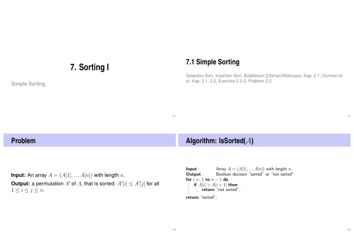
7.1 Simple Sorting 7. Sorting I Selection Sort, Insertion Sort, Bubblesort [Ottman/Widmayer, Kap. 2.1, Cormen et al, Kap. 2.1, 2.2, Exercise 2.2-2, Problem 2-2 Simple Sorting 196 197 Algorithm: IsSorted( A ) Problem Input : Array A = ( A [1] , ..., A [ n ]) with length n . Output : Boolean decision “sorted” or “not sorted” Input: An array A = ( A [1] , ..., A [ n ]) with length n . for i ← 1 to n − 1 do Output: a permutation A ′ of A , that is sorted: A ′ [ i ] ≤ A ′ [ j ] for all if A [ i ] > A [ i + 1] then 1 ≤ i ≤ j ≤ n . return “not sorted”; return “sorted”; 198 199

Observation Give it a try 5 6 2 8 4 1 ( j = 1) IsSorted( A ):“not sorted”, if A [ i ] > A [ i + 1] for an i . 5 6 2 8 4 1 ( j = 2) Not sorted! . ⇒ idea: 5 2 6 8 4 1 ( j = 3) But the greatest for j ← 1 to n − 1 do element moves to the if A [ j ] > A [ j + 1] then 5 2 6 8 4 1 ( j = 4) right swap( A [ j ] , A [ j + 1] ); ⇒ new idea! 5 2 6 4 8 1 ( j = 5) 5 2 6 4 1 8 200 201 Try it out Algorithm: Bubblesort ( j = 1 , i = 1) 5 6 2 8 4 1 5 6 2 8 4 1 ( j = 2) ( j = 3) 5 2 6 8 4 1 Input : Array A = ( A [1] , . . . , A [ n ]) , n ≥ 0 . Apply the procedure 5 2 6 8 4 1 ( j = 4) Output : Sorted Array A ( j = 5) 5 2 6 4 8 1 iteratively. 5 2 6 4 1 8 ( j = 1 , i = 2) for i ← 1 to n − 1 do ( j = 2) 2 5 6 4 1 8 For A [1 , . . . , n ] , for j ← 1 to n − i do 2 5 6 4 1 8 ( j = 3) ( j = 4) if A [ j ] > A [ j + 1] then 2 5 4 6 1 8 then A [1 , . . . , n − 1] , 2 5 4 1 6 8 ( j = 1 , i = 3) swap( A [ j ] , A [ j + 1] ); ( j = 2) 2 5 4 1 6 8 then A [1 , . . . , n − 2] , 2 4 5 1 6 8 ( j = 3) ( j = 1 , i = 4) etc. 2 4 1 5 6 8 2 4 1 5 6 8 ( j = 2) ( i = 1 , j = 5) 2 1 4 5 6 8 1 2 4 5 6 8 202 203

Analysis Selection Sort Number key comparisons � n − 1 i =1 ( n − i ) = n ( n − 1) = Θ( n 2 ) . ( i = 1) 5 6 2 8 4 1 2 Number swaps in the worst case: Θ( n 2 ) 1 6 2 8 4 5 ( i = 2) Iterative procedure ? What is the worst case? as for Bubblesort. 1 2 6 8 4 5 ( i = 3) Selection of the ! If A is sorted in decreasing order. 1 2 4 8 6 5 ( i = 4) smallest (or largest) 1 2 4 5 6 8 ( i = 5) element by ? Algorithm can be adapted such that it terminates when the array is sorted. immediate search. 1 2 4 5 6 8 ( i = 6) Key comparisons and swaps of the modified algorithm in the best case? 1 2 4 5 6 8 ! Key comparisons = n − 1 . Swaps = 0 . 204 205 Algorithm: Selection Sort Analysis Input : Array A = ( A [1] , . . . , A [ n ]) , n ≥ 0 . Output : Sorted Array A Number comparisons in worst case: Θ( n 2 ) . for i ← 1 to n − 1 do p ← i Number swaps in the worst case: n − 1 = Θ( n ) for j ← i + 1 to n do if A [ j ] < A [ p ] then Best case number comparisons: Θ( n 2 ) . p ← j ; swap( A [ i ] , A [ p ] ) 206 207

Insertion Sort Insertion Sort ( i = 1) 5 6 2 8 4 1 ? What is the disadvantage of this algorithm compared to sorting Iterative procedure: by selection? 5 6 2 8 4 1 ( i = 2) i = 1 ...n ! Many element movements in the worst case. 5 6 2 8 4 1 ( i = 3) Determine insertion position for element i . 2 5 6 8 4 1 ( i = 4) ? What is the advantage of this algorithm compared to selection Insert element i array 2 5 6 8 4 1 ( i = 5) sort? block movement 2 4 5 6 8 1 ( i = 6) ! The search domain (insertion interval) is already sorted. potentially required Consequently: binary search possible. 1 2 4 5 6 8 208 209 Algorithm: Insertion Sort Analysis Input : Array A = ( A [1] , . . . , A [ n ]) , n ≥ 0 . Output : Sorted Array A Number comparisons in the worst case: for i ← 2 to n do � n − 1 k =1 a · log k = a log(( n − 1)!) ∈ O ( n log n ) . x ← A [ i ] Number comparisons in the best case Θ( n log n ) . 4 p ← BinarySearch( A [1 ...i − 1] , x ); // Smallest p ∈ [1 , i ] with A [ p ] ≥ x for j ← i − 1 downto p do Number swaps in the worst case � n k =2 ( k − 1) ∈ Θ( n 2 ) A [ j + 1] ← A [ j ] A [ p ] ← x 4 With slight modification of the function BinarySearch for the minimum / maximum: Θ( n ) 210 211

Different point of view Different point of view 5 5 Sorting node: 6 ≷ 6 6 5 4 2 5 2 ≷ ≷ 6 5 2 Like selection sort 8 8 8 8 ≷ ≷ ≷ 8 8 ≷ 8 [and like Bubblesort] 2 5 6 4 4 5 6 ≷ ≷ ≷ ≷ 4 8 4 2 4 5 6 1 2 4 5 6 ≷ ≷ ≷ ≷ ≷ 1 8 1 2 4 5 6 5 1 2 4 6 8 212 213 Different point of view Conclusion 5 5 6 6 ≷ 6 5 2 5 ≷ ≷ 2 In a certain sense, Selection Sort, Bubble Sort and Insertion Sort 6 provide the same kind of sort strategy. Will be made more precise. 5 2 5 8 8 8 ≷ ≷ ≷ 8 Like insertion sort 8 2 5 6 4 4 5 6 ≷ ≷ ≷ ≷ 4 8 2 4 5 6 1 2 4 5 6 ≷ ≷ ≷ ≷ ≷ 1 8 5 6 1 2 4 1 2 4 5 6 8 5 In the part about parallel sorting networks. For the sequential code of course the observations as described above still hold. 214 215

Shellsort Shellsort 9 8 7 6 5 4 3 2 1 0 insertion sort, k = 4 1 8 7 6 5 4 3 2 9 0 Insertion sort on subsequences of the form ( A k · i ) ( i ∈ ◆ ) with 1 0 7 6 5 4 3 2 9 8 decreasing distances k . Last considered distance must be k = 1 . 1 0 3 6 5 4 7 2 9 8 Good sequences: for example sequences with distances 1 0 3 2 5 4 7 6 9 8 k ∈ { 2 i 3 j | 0 ≤ i, j } . insertion sort, k = 2 1 0 3 2 5 4 7 6 9 8 1 0 3 2 5 4 7 6 9 8 insertion sort, k = 1 0 1 2 3 4 5 6 7 8 9 216 217 8.1 Heapsort 8. Sorting II [Ottman/Widmayer, Kap. 2.3, Cormen et al, Kap. 6] Heapsort, Quicksort, Mergesort 218 219

[Max-]Heap 6 Heapsort Binary tree with the following prop- Wurzel erties 1 complete up to the lowest Inspiration from selectsort: fast insertion 22 level Inspiration from insertion sort: fast determination of position parent 20 18 2 Gaps (if any) of the tree in ? Can we have the best of both worlds? the last level to the right child 16 12 15 17 3 Heap-Condition: ! Yes, but it requires some more thinking... Max-(Min-)Heap: key of a 3 2 8 11 14 child smaller (greater) thant leaves that of the parent node 6 Heap(data structure), not: as in “heap and stack” (memory allocation) 220 221 Heap and Array Recursive heap structure Tree → Array: A heap consists of two heaps: 22 children ( i ) = { 2 i, 2 i + 1 } [1] parent ( i ) = ⌊ i/ 2 ⌋ 20 18 22 [2] [3] Vater 16 12 15 17 20 18 [4] [5] [6] [7] 22 20 18 16 12 15 17 3 2 8 11 14 3 2 8 11 14 16 12 15 17 1 2 3 4 5 6 7 8 9 10 11 12 [8] [9] [10] [11] [12] Kinder 3 2 8 11 14 Depends on the starting index 7 7 For array that start at 0 : { 2 i, 2 i + 1 } → { 2 i + 1 , 2 i + 2 } , ⌊ i/ 2 ⌋ → ⌊ ( i − 1) / 2 ⌋ 222 223

Insert Remove the maximum 22 21 20 18 20 18 Replace the maximum by the lower Insert new element at the first free right element 16 12 15 17 16 12 15 17 position. Potentially violates the heap Reestablish heap property: sink property. 3 2 8 11 14 3 2 8 11 14 successively (in the direction of the Reestablish heap property: climb 22 20 greater child) successively Worst case number of operations: 20 21 16 18 Worst case number of operations: O (log n ) O (log n ) 16 18 12 17 14 12 15 17 3 2 8 11 14 15 3 2 8 11 224 225 Algorithm Sink( A, i, m ) Sort heap 7 6 4 5 1 2 Input : Array A with heap structure for the children of i . Last element m . 2 6 4 5 1 7 ⇒ Output : Array A with heap structure for i with last element m . swap while 2 i ≤ m do ⇒ 6 5 4 2 1 7 sink j ← 2 i ; // j left child A [1 , ..., n ] is a Heap. 1 5 4 2 6 7 swap ⇒ if j < m and A [ j ] < A [ j + 1] then While n > 1 j ← j + 1 ; // j right child with greater key 5 7 ⇒ 4 2 1 6 sink swap( A [1] , A [ n ] ) if A [ i ] < A [ j ] then 1 4 2 5 6 7 swap ⇒ Sink( A, 1 , n − 1 ); swap( A [ i ] , A [ j ] ) 4 1 2 5 6 7 ⇒ sink i ← j ; // keep sinking n ← n − 1 ⇒ 2 1 4 5 6 7 swap else i ← m ; // sinking finished 2 1 4 5 6 7 sink ⇒ 5 7 ⇒ 1 2 4 6 swap 226 227

Algorithm HeapSort( A, n ) Heap creation Input : Array A with length n . Output : A sorted. // Build the heap. Observation: Every leaf of a heap is trivially a correct heap. for i ← n/ 2 downto 1 do Sink( A, i, n ); // Now A is a heap. for i ← n downto 2 do Consequence: Induction from below! swap( A [1] , A [ i ] ) Sink( A, 1 , i − 1 ) // Now A is sorted. 228 229 Analysis: sorting a heap Analysis: creating a heap Calls to sink: n/ 2 . Thus number of comparisons and movements: v ( n ) ∈ O ( n log n ) . But mean length of sinking paths is much smaller: Sink traverses at most log n nodes. For each node 2 key � n comparisons. ⇒ sorting a heap costs in the worst case 2 log n ⌊ log n ⌋ ⌊ log n ⌋ � h � � v ( n ) = · c · h ∈ O ( n 2 h ) comparisons. 2 h +1 h =0 h =0 Number of memory movements of sorting a heap also O ( n log n ) . k =0 kx k = with s ( x ) := � ∞ (0 < x < 1) 8 and s ( 1 x 2 ) = 2 : (1 − x ) 2 v ( n ) ∈ O ( n ) . 8 f ( x ) = 1 − x = 1 + x + x 2 ... ⇒ f ′ ( x ) = 1 1 (1 − x ) 2 = 1 + 2 x + ... 230 231