15-780: LinearProgramming J. Zico Kolter February 1-3, 2016 1 - PowerPoint PPT Presentation

15-780: Linear Programming J. Zico Kolter February 1-3, 2016 1

Outline Introduction Some linear algebra review Linear programming Simplex algorithm Duality and dual simplex 2

Outline Introduction Some linear algebra review Linear programming Simplex algorithm Duality and dual simplex 3

Decision-making with continuous variables The problems we have focused on thus far in class have usually involved making discrete assignments to variables An amazing property: Discrete search (Convex) optimization Variables discrete continuous real-valued # possible solutions finite infinite Complexity of solving exponential polynomial Techniques developed in Operations Research / Engineering communities, one of the biggest trends of the past ~15 years has been the integration into AI work 4

Example: manufacturing A large factory makes tables and chairs. Each table returns a profit of $200 and each chair a profit of $100. Each table takes 1 unit of metal and 3 units of wood and each chair takes 2 units of metal and 1 unit of wood. The factory has 6K units of metal and 9K units of wood. How many tables and chairs should the factory make to maximize profit? 5

Example: manufacturing A large factory makes tables and chairs. Each table returns a profit of $200 and each chair a profit of $100. Each table takes 1 unit of metal and 3 units of wood and each chair takes 2 units of metal and 1 unit of wood. The factory has 6K units of metal and 9K units of wood. How many tables and chairs should the factory make to maximize profit? x 2 (chairs) x 1 (tables) 5

Example: manufacturing A large factory makes tables and chairs. Each table returns a profit of $200 and each chair a profit of $100. Each table takes 1 unit of metal and 3 units of wood and each chair takes 2 units of metal and 1 unit of wood. The factory has 6K units of metal and 9K units of wood. How many tables and chairs should the factory make to maximize profit? x 2 (chairs) x 1 + 2 x 2 ≤ 6 (metal) x 1 (tables) 5

Example: manufacturing A large factory makes tables and chairs. Each table returns a profit of $200 and each chair a profit of $100. Each table takes 1 unit of metal and 3 units of wood and each chair takes 2 units of metal and 1 unit of wood. The factory has 6K units of metal and 9K units of wood. How many tables and chairs should the factory make to maximize profit? x 2 (chairs) 3 x 1 + x 2 ≤ 9 (wood) x 1 + 2 x 2 ≤ 6 (metal) x 1 (tables) 5

Example: manufacturing A large factory makes tables and chairs. Each table returns a profit of $200 and each chair a profit of $100. Each table takes 1 unit of metal and 3 units of wood and each chair takes 2 units of metal and 1 unit of wood. The factory has 6K units of metal and 9K units of wood. How many tables and chairs should the factory make to maximize profit? x 2 (chairs) 3 x 1 + x 2 ≤ 9 (wood) Profit = 2 x 1 + x 2 x 1 + 2 x 2 ≤ 6 (metal) x 1 (tables) 5

Example: manufacturing A large factory makes tables and chairs. Each table returns a profit of $200 and each chair a profit of $100. Each table takes 1 unit of metal and 3 units of wood and each chair takes 2 units of metal and 1 unit of wood. The factory has 6K units of metal and 9K units of wood. How many tables and chairs should the factory make to maximize profit? x 2 (chairs) 3 x 1 + x 2 ≤ 9 (wood) x ⋆ 1 = 2 . 4 , x ⋆ 2 = 1 . 8 Profit = 2 x 1 + x 2 x 1 + 2 x 2 ≤ 6 (metal) x 1 (tables) 5

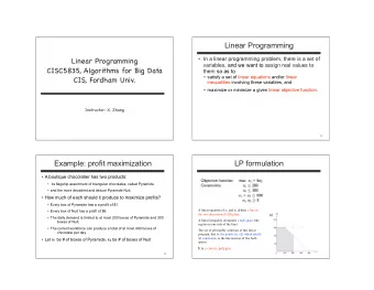
maximize Example: manufacturing A large factory makes tables and chairs. Each table returns a profit of $200 and each chair a profit of $100. Each table takes 1 unit of metal and 3 units of wood and each chair takes 2 units of metal and 1 unit of wood. The factory has 6K units of metal and 9K units of wood. How many tables and chairs should the factory make to maximize profit? 2 x 1 + x 2 x 1 , x 2 subject to x 1 + 2 x 2 ≤ 6 3 x 1 + x 2 ≤ 9 x 1 , x 2 ≥ 0 5

Other examples 1. Solve tree-structured CSPs 2. Finding optimal strategies for two player, zero sum games 3. Finding most probable assignment in a graphical model 4. Finding (or approximating) solution of a Markov decision problem 5. Min-cut / max-flow network problems 6. Applications: economic portfolio optimization, robotic control, scheduling generation in smart grids, many many others 6

Comments Not covered at all in textbook, lecture notes + video + supplementary material on class page is enough to complete all assignments But, if you want a more thorough reference, you can look at: Bertsimas and Tsitsiklis, “Introduction to Linear Optimization”, Chapters 1-5. Part of a much broader class of “tractable” optimization problems: convex optimization problems (we’ll return to more general problems and other optimization techniques later in the course) 7

Outline Introduction Some linear algebra review Linear programming Simplex algorithm Duality and dual simplex 8

http://www.cs.cmu.edu/~zkolter/course/linalg Linear algebra Throughout this lecture we’re going to use matrix and vector notation to describe linear programming problems This is very basic linear algebra (nothing more complex than addition, multiplication, and inverses) But, if you’re not familiar with linear algebra notation, it will be confusing, you can take a look at these lectures for some review: 9

Vectors We use the notation x ∈ R n to denote a vector with n entries x i denotes the i th element of x By convention, x ∈ R n represents a column vector (a matrix with one column and n rows); to indicate a row vector, we use x T ( x transpose)   x 1 x 2   x T = [ ] x = . x 1 x 2 · · · x n    , .  .   x n 10

Matrices We use the notation A ∈ R m × n to denote a matrix with m rows and n columns We use a ij (or sometimes A ij , a i , j , etc) to denote the entry in the i th row and j th column; we use a i to refer to the i th column of A , and a T to refer to the i th row of A i    — a T —  a 11 · · · a 1 n   | | 1 . . . ... . .  = . A =  = · · · a 1 a n  . .   .      | | — a T — a m 1 · · · a mn m 11

Addition/subtraction and transposes Addition and subtraction of matrices and vectors is defined just as addition or subtraction of the elements, for A , B ∈ R m × n , C ∈ R m × n = A + B ⇐ ⇒ c ij = a ij + b ij Transpose operation switches rows and columns D ∈ R n × m = A T ⇐ ⇒ d ij = a ji 12

Matrix multiplication For two matrices A ∈ R m × n , B ∈ R m × p , n C ∈ R n × p = AB ∑ ⇐ ⇒ c ij = a ik b kj k =1 Special case: inner product of two vectors, for x , y ∈ R n n x T y ∈ R = ∑ x i y i i =1 Special case: product of matrix and vector, for A ∈ R m × n , x ∈ R n  a T  1 x n . Ax ∈ R m = . ∑  = a i x i .    a T i =1 m x 13

Matrix multiplication properties Associative: A ( BC ) = ( AB ) C Distributive: A ( B + C ) = AB + AC Not commutative: AB ̸ = BA Transpose of product: ( AB ) T = B T A T 14

Matrix inverse Identity matrix I ∈ R n × n is a square matrix with ones on diagonal and zeros elsewhere; has property that for any A ∈ R m × n IA = A , AI = A , (for different sized I matrices) For a square matrix A ∈ R n × n , inverse A − 1 is th matrix such that A − 1 A = I = AA − 1 Properties: - May not exists even for square matrices (linear independence and rank conditions) - ( AB ) − 1 = B − 1 A − 1 if A and B are square and invertible - ( A − 1 ) T = ( A T ) − 1 ≡ A − T 15

Vector norms For x ∈ R n , we’ll use ∥ x ∥ 2 to denote the Euclidean norm of x � n √ � ∑ � x 2 x T x ∥ x ∥ 2 = i = � i =1 n (and also) ∥ x ∥ 2 ∑ x 2 i = x T x 2 = i =1 Thus, for two vectors x , y ∈ R n , ∥ x − y ∥ 2 denotes the Euclidean distance between x and y � n � ∑ ( x i − y i ) 2 = √ � x T x + y T y − 2 x T y ∥ x − y ∥ 2 = � i =1 The 2 subscript denotes the fact that this is called the 2-norm of a vector, we’ll see other norms like the 1-norm and ∞ -norm 16

Outline Introduction Some linear algebra review Linear programming Simplex algorithm Duality and dual simplex 17

maximize Example: manufacturing Let’s return to the example we started with: x 2 (chairs) 2 x 1 + x 2 3 x 1 + x 2 ≤ 9 (wood) x 1 , x 2 subject to x 1 + 2 x 2 ≤ 6 Profit = 2 x 1 + x 2 3 x 1 + x 2 ≤ 9 x 1 + 2 x 2 ≤ 6 (metal) x 1 , x 2 ≥ 0 x 1 (tables) 18

maximize maximize subject to Inequality form linear programs Using linear algebra notation, we can write linear program more compactly as c T x x subject to Gx ≤ h with optimization variable x ∈ R n and problem data c ∈ R n , G ∈ R m × n , and h ∈ R m and where the ≤ denotes elementwise inequality (equality constraints also possible: g T i x = h i ≡ g T i x ≤ h i , − g T i x ≤ h i ) Example in inequality form: 2 x 1 + x 2     1 2 6 [ 2 x 1 , x 2 ] 3 1 9 x 1 + 2 x 2 ≤ 6     c = G =  h =     1 − 1 0 0 3 x 1 + x 2 ≤ 9    0 − 1 0 x 1 , x 2 ≥ 0 19

maximize Geometry of linear programs Consider the inequality constraints of the linear program written out explicitly c T x x subject to g T i x ≤ h i , i = 1 , . . . , m Each constraint g T i x ≤ h i represents a halfspace constraint x 2 g i h i ∥ g i ∥ 2 x 1 20