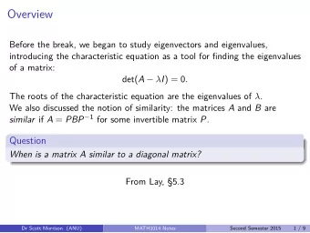
lgebra Linear e Aplicaes EIGENVALUES AND EIGENVECTORS Motivation #1 - PowerPoint PPT Presentation

Álgebra Linear e Aplicações

EIGENVALUES AND EIGENVECTORS

Motivation #1 • We have so far been focusing on systems of linear algebraic equations • We now move on to study systems of linear differential equations du 1 = 7 u 1 − 4 u 2 ✓ u 0 ◆ ✓ 7 ◆ ✓ u 1 ◆ dt − 4 u 0 = Au 1 = du 2 u 0 5 − 2 u 2 2 = 5 u 1 − 2 u 2 dt • Solutions to are of the form u = α e λ t u 0 = λ u • This motivates us to seek solutions in the same form

Motivation #2 • Substituting and we get u 2 = α 2 e λ t u 1 = α 1 e λ t du 1 λα 1 e λ t = 7 α 1 e λ t − 4 α 2 e λ t = 7 u 1 − 4 u 2 λα 1 = 7 α 1 − 4 α 2 dt ⇒ ⇒ du 2 λα 2 e λ t = 5 α 1 e λ t − 2 α 2 e λ t λα 2 = 5 α 1 − 2 α 2 = 5 u 1 − 2 u 2 dt • In other words, ✓ 7 ◆ ✓ α 1 ◆ ✓ α 1 ◆ − 4 ✓ α 1 ◆ = λ with ⇒ Ax = λ x x = 5 − 2 α 2 α 2 α 2 • Each pair , with nonzero x , gives us a solution ( λ , x ) to the differential equation in the form we sought

Eigenvectors and Eigenvalues • For an n × n matrix A , scalars and vectors x n × 1 ≠ 0 λ such that are called eigenvalues and Ax = λ x eigenvectors of A , respectively • Each pair is called an eigenpair ( λ , x ) • The set of distinct eigenvalues, denoted by , is σ ( A ) called the spectrum of A is singular • ⇔ det( A − λ I ) = 0 λ ∈ σ ( A ) ⇔ A − λ I , the set of eigenvectors • { x 6 = 0 | x 2 N ( A � λ I ) } associated to , is an eigenspace for A λ • Nonzero row vectors such that are y ∗ ( A − λ I ) = 0 y ∗ called left-hand eigenvectors for A

Geometrically • Eigenvectors experience only change in magnitude or sign under transformation by A Ax Ax = λ x x x generic vector x eigenvector x

Back to Motivation #1 • Let us find the eigenvalues of matrix A in our differential equation ✓ u 0 ◆ ✓ 7 ◆ ✓ u 1 ◆ − 4 u 0 = Au 1 = u 0 5 − 2 u 2 2 must be singular, so • A − λ I � � 7 − λ − 4 � = 0 ⇒ p ( λ ) = λ 2 − 5 λ + 6 = 0 � � det( A − λ I ) = 0 ⇒ � � 5 − 2 − λ � • Eigenvalues and make singular λ = 2 λ = 3 A − λ I • To find the eigenvectors, find and N ( A − 2 I ) N ( A − 3 I ) ✓ 5 ◆ ✓ 4 ◆ − 4 − 4 ( A − 2 I ) x = 0 ⇒ x = 0 ( A − 3 I ) x = 0 ⇒ x = 0 5 − 4 5 − 5 ✓ 4 ◆ ✓ 1 ◆ x = α x = β 5 1

Back to Motivation #2 • Each eigenpair leads to an independent solution ✓ ◆ ✓ ◆ 4 1 u 1 = e λ 1 t x 1 = e 2 t u 2 = e λ 2 t x 2 = e 3 t 5 1 • Linear combinations of u 1 and u 2 are also solutions • In fact, all solutions are linear combinations of u 1 and u 2 du 1 u 1 = α 1 4 e 2 t + α 2 e 3 t = 7 u 1 − 4 u 2 dt ⇒ du 2 u 2 = α 1 5 e 2 t + α 2 e 3 t = 5 u 1 − 2 u 2 dt

Characteristic Polynomial and Equation • The characteristic polynomial of A n × n is p ( λ ) = det( A − λ I ) • The degree is n and the leading term is ( − 1) n λ n • The characteristic equation for A is p ( λ ) = 0 • The eigenvalues of A are the solutions of the characteristic equation, i.e., the roots of the characteristic polynomial • Altogether, A has n eigenvalues, but some may be complex numbers (even if A is real) and some may be repeated • If A is real, then its complex eigenvalues must appear in conjugate pairs. I.e., if then ¯ λ ∈ σ ( A ) λ ∈ σ ( A )

The Companion Matrix • Consider the following matrix   0 0 0 − a 0 · · · 1 0 0 − a 1 · · ·     0 1 0 − a 2 A p = · · ·     . . . . ... . . . .   . . . .   0 0 1 − a n − 1 · · · • It’s monic characteristic polynomial is det( x I − A p ) = p ( x ) = a 0 + a 1 x + a 2 x 2 + · · · + a n − 1 x n − 1 + x n • Proof: expand by minors on the last column

Poor man’s root finder • Assume there is some magical finite eigenvalue-finding algorithm • We can take any polynomial, build its companion matrix, and feed to it • This would give us the roots of any polynomial • But there is no magical root-finding algorithm • So there can’t be a magical eigenvalue-finding algorithm either

DIAGONALIZATION BY SIMILARITY TRANSFORMATIONS

Example of Diagonalization • A good choice of coordinate system (basis) can significantly simplify an equation or problem • Consider the oblique ellipse 13 x 2 + 10 xy + 13 y 2 = 72 y � ✓ 13 ◆ ✓ x ◆ 5 � x = 72 5 13 y y ✓ x ◆ ✓ 1 ◆ ✓ u ◆ 1 1 = u √ 1 − 1 y 2 v ◆ 1 ◆ 1 v � ✓ 1 ✓ 13 ✓ 1 ◆ ✓ u ◆ 1 5 1 � u = 72 √ √ x 1 − 1 5 13 1 − 1 2 2 v v � ✓ 18 ◆ ✓ u ◆ 0 v � u = 72 0 8 v • No cross-term in new coordinates: u 2 4 + v 2 9 = 1

Similarities revisited • Matrices A n × n and B n × n are said to be similar matrices whenever there exists a nonsingular matrix P such that P – 1 AP = B . The product P – 1 AP is called a similarity transformation on A • Similarities preserve the characteristic polynomial P − 1 ( A − λ I ) P det( B − λ I ) = det( P − 1 AP − λ I ) = det � � = det( P − 1 ) det( A − λ I ) det( P ) = det( A − λ I ) • Similar matrices share the same eigenvalues • Eigenvalues are intrinsic to the linear operator • Eigenvectors depend on coordinate system • Row reductions do not preserve eigenvalues

A Fundamental Problem • Given a square matrix A , reduce it to the simplest possible form by means of a similarity • Diagonal matrices are the simplest • Are all matrices similar to a diagonal matrix? ✓ 0 ◆ 1 P − 1 AP = D ⇒ P − 1 APP − 1 AP = D 2 A = 0 0 ⇒ P − 1 A 2 P = D 2 ⇒ 0 = D 2 A 2 = 0 ⇒ A = 0 • So no, certainly not for nilpotent matrices • Can we at least triangularize?

Schur’s Triangularization Theorem • Every square matrix is unitarily similar to an upper-triangular matrix • I.e., for each A n × n there is an unitary matrix U and an upper-triangular matrix T such that U – 1 AU = T • Proof by induction • Basis: If a matrix is 1 × 1 , nothing needs to be done • Assumption: Every n – 1 × n – 1 matrix can be triangularized • Induction step: Prove n × n matrix can be triangularized ✓ λ ◆ Ax = λ x � x X � a ∗ Q U = ◆ ( UV ) ∗ AUV = 0 Q ∗ BQ ✓ x ∗ Ax ◆ ✓ λ x ∗ AX a ∗ U ∗ AU = = X ∗ Ax X ∗ AX ✓ λ ◆ 0 B n − 1 × n − 1 a ∗ Q = T = ˜ 0 T ✓ 1 ◆ 0 B = Q ∗ ˜ TQ V = 0 Q