Overview The previous lecture introduced eigenvalues and - PowerPoint PPT Presentation
Overview The previous lecture introduced eigenvalues and eigenvectors. Well review these definitions before considering the following question: Question Given a square matrix A, how can you find the eigenvalues of A? Well discuss an
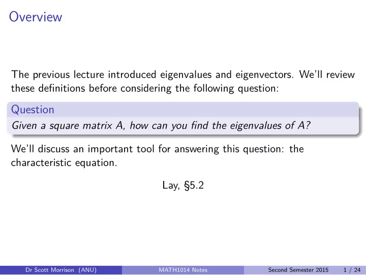
Overview The previous lecture introduced eigenvalues and eigenvectors. We’ll review these definitions before considering the following question: Question Given a square matrix A, how can you find the eigenvalues of A? We’ll discuss an important tool for answering this question: the characteristic equation. Lay, §5.2 Dr Scott Morrison (ANU) MATH1014 Notes Second Semester 2015 1 / 24
Eigenvalues and eigenvectors Definition An eigenvector of an n × n matrix A is a non-zero vector x such that A x = λ x for some scalar λ . The scalar λ is an eigenvalue for A . Dr Scott Morrison (ANU) MATH1014 Notes Second Semester 2015 2 / 24
Eigenvalues and eigenvectors Definition An eigenvector of an n × n matrix A is a non-zero vector x such that A x = λ x for some scalar λ . The scalar λ is an eigenvalue for A . Multiplying a vector by a matrix changes the vector. An eigenvector is a vector which is changed in the simplest way: by scaling. Dr Scott Morrison (ANU) MATH1014 Notes Second Semester 2015 2 / 24
Eigenvalues and eigenvectors Definition An eigenvector of an n × n matrix A is a non-zero vector x such that A x = λ x for some scalar λ . The scalar λ is an eigenvalue for A . Multiplying a vector by a matrix changes the vector. An eigenvector is a vector which is changed in the simplest way: by scaling. Given any matrix, we can study the associated linear transformation. One way to understand this function is by identifying the set of vectors for which the transformation is just scalar multiplication. Dr Scott Morrison (ANU) MATH1014 Notes Second Semester 2015 2 / 24
Example Example 1 � � 2 1 Let A = . 0 − 1 � � 1 Then u = is an eigenvector for the eigenvalue 2: 0 � � � � � � 2 1 1 2 A u = = = 2 u . 0 − 1 0 0 � � 1 Also, v = is an eigenvector for the eigenvalue − 1: − 3 � � � � � � 2 1 1 − 1 A v = = = − v . 0 − 1 − 3 3 Dr Scott Morrison (ANU) MATH1014 Notes Second Semester 2015 3 / 24
Finding Eigenvalues Suppose we know that λ ∈ R is an eigenvalue for A . That is, for some x � = 0 , A x = λ x . Then we solve for an eigenvector x by solving ( A − λ I ) x = 0 . But how do we find eigenvalues in the first place? Dr Scott Morrison (ANU) MATH1014 Notes Second Semester 2015 4 / 24
Finding Eigenvalues Suppose we know that λ ∈ R is an eigenvalue for A . That is, for some x � = 0 , A x = λ x . Then we solve for an eigenvector x by solving ( A − λ I ) x = 0 . But how do we find eigenvalues in the first place? x must be non zero ⇓ ( A − λ I ) x = 0 must have non trivial solutions ⇓ ( A − λ I ) is not invertible ⇓ det( A − λ I ) = 0. Dr Scott Morrison (ANU) MATH1014 Notes Second Semester 2015 4 / 24
Finding Eigenvalues Suppose we know that λ ∈ R is an eigenvalue for A . That is, for some x � = 0 , A x = λ x . Then we solve for an eigenvector x by solving ( A − λ I ) x = 0 . But how do we find eigenvalues in the first place? x must be non zero ⇓ ( A − λ I ) x = 0 must have non trivial solutions ⇓ ( A − λ I ) is not invertible ⇓ det( A − λ I ) = 0. Solve det( A − λ I ) = 0 for λ to find the eigenvalues of the matrix A . Dr Scott Morrison (ANU) MATH1014 Notes Second Semester 2015 4 / 24
The eigenvalues of a square matrix A are the solutions of the characteristic equation. the characteristic polynomial : det( A − λ I ) the characteristic equation : det( A − λ I ) = 0 Dr Scott Morrison (ANU) MATH1014 Notes Second Semester 2015 5 / 24
Examples Example 2 Consider the matrix � � 5 3 A = . 3 5 We want to find the eigenvalues of A . Dr Scott Morrison (ANU) MATH1014 Notes Second Semester 2015 6 / 24
Examples Example 2 Consider the matrix � � 5 3 A = . 3 5 We want to find the eigenvalues of A . Since � � � � � � 5 3 λ 0 5 − λ 3 A − λ I = − = , 3 5 0 λ 3 5 − λ Dr Scott Morrison (ANU) MATH1014 Notes Second Semester 2015 6 / 24
Examples Example 2 Consider the matrix � � 5 3 A = . 3 5 We want to find the eigenvalues of A . Since � � � � � � 5 3 λ 0 5 − λ 3 A − λ I = − = , 3 5 0 λ 3 5 − λ The equation det( A − λ I ) = 0 becomes (5 − λ )(5 − λ ) − 9 = 0 λ 2 − 10 λ + 16 = 0 ( λ − 8)( λ − 2) = 0 ⇒ λ = 2 , λ = 8 . Dr Scott Morrison (ANU) MATH1014 Notes Second Semester 2015 6 / 24
Example 3 Find the characteristic equation for the matrix 0 3 1 A = 3 0 2 . 1 2 0 Dr Scott Morrison (ANU) MATH1014 Notes Second Semester 2015 7 / 24
Example 3 Find the characteristic equation for the matrix 0 3 1 A = 3 0 2 . 1 2 0 For a 3 × 3 matrix, recall that a determinant can be computed by cofactor expansion. − λ 3 1 A − λ I = 3 − λ 2 1 2 − λ Dr Scott Morrison (ANU) MATH1014 Notes Second Semester 2015 7 / 24
− λ 3 1 det( A − λ I ) = det 3 − λ 2 1 2 − λ � � � � � � − λ 2 3 2 3 − λ � � � � � � = − λ � − 3 � + 1 � � � � � � 2 − λ 1 − λ 1 2 � � � � � � � � � � − λ ( λ 2 − 4) − 3( − 3 λ − 2) + (6 + λ ) = − λ 3 + 4 λ + 9 λ + 6 + 6 + λ = − λ 3 + 14 λ + 12 = Hence the characteristic equation is − λ 3 + 14 λ + 12 = 0 . The eigenvalues of A are the solutions to the characteristic equation. Dr Scott Morrison (ANU) MATH1014 Notes Second Semester 2015 8 / 24
Example 4 Consider the matrix 3 0 0 0 0 2 1 0 0 0 A = − 1 4 2 0 0 8 6 − 3 0 0 5 − 2 4 − 1 1 Find the characteristic equation for this matrix. Dr Scott Morrison (ANU) MATH1014 Notes Second Semester 2015 9 / 24
Observe that 3 − λ 0 0 0 0 2 1 − λ 0 0 0 det( A − λ I ) = − 1 4 2 − λ 0 0 8 6 − 3 − λ 0 5 − 2 4 − 1 1 − λ = (3 − λ )(1 − λ )(2 − λ )( − λ )(1 − λ ) ( − λ )(1 − λ ) 2 (3 − λ )(2 − λ ) = Dr Scott Morrison (ANU) MATH1014 Notes Second Semester 2015 10 / 24
Observe that 3 − λ 0 0 0 0 2 1 − λ 0 0 0 det( A − λ I ) = − 1 4 2 − λ 0 0 8 6 − 3 − λ 0 5 − 2 4 − 1 1 − λ = (3 − λ )(1 − λ )(2 − λ )( − λ )(1 − λ ) ( − λ )(1 − λ ) 2 (3 − λ )(2 − λ ) = Thus A has eigenvalues 0 , 1 , 2 and 3. The eigenvalue 1 is said to have multiplicity 2 because the factor 1 − λ occurs twice in the characteristic polynomial. Dr Scott Morrison (ANU) MATH1014 Notes Second Semester 2015 10 / 24
Observe that 3 − λ 0 0 0 0 2 1 − λ 0 0 0 det( A − λ I ) = − 1 4 2 − λ 0 0 8 6 − 3 − λ 0 5 − 2 4 − 1 1 − λ = (3 − λ )(1 − λ )(2 − λ )( − λ )(1 − λ ) ( − λ )(1 − λ ) 2 (3 − λ )(2 − λ ) = Thus A has eigenvalues 0 , 1 , 2 and 3. The eigenvalue 1 is said to have multiplicity 2 because the factor 1 − λ occurs twice in the characteristic polynomial. In general the (algebraic) multiplicity of an eigenvalue λ is its multiplicity as a root of the characteristic equation. Dr Scott Morrison (ANU) MATH1014 Notes Second Semester 2015 10 / 24
Similarity The next theorem illustrates the use of the characteristic polynomial, and it provides a basis for several iterative methods that approximate eigenvalues. Definition (Similar matrices) If A and B are n × n matrices, then A is similar to B if there is an invertible matrix P such that P − 1 AP = B or equivalently, A = PBP − 1 . We say that A and B are similar . Changing A into P − 1 AP is called a similarity transformation . Dr Scott Morrison (ANU) MATH1014 Notes Second Semester 2015 11 / 24
Theorem If the n × n matrices A and B are similar, then they have the same characteristic polynomial and hence the same eigenvalues (with the same multiplicities). Dr Scott Morrison (ANU) MATH1014 Notes Second Semester 2015 12 / 24
Theorem If the n × n matrices A and B are similar, then they have the same characteristic polynomial and hence the same eigenvalues (with the same multiplicities). Proof. If B = P − 1 AP , then P − 1 AP − λ P − 1 P B − λ I = P − 1 ( AP − λ P ) = P − 1 ( A − λ I ) P . = Hence � � P − 1 ( A − λ I ) P det( B − λ I ) = det Dr Scott Morrison (ANU) MATH1014 Notes Second Semester 2015 12 / 24
Theorem If the n × n matrices A and B are similar, then they have the same characteristic polynomial and hence the same eigenvalues (with the same multiplicities). Proof. If B = P − 1 AP , then P − 1 AP − λ P − 1 P B − λ I = P − 1 ( AP − λ P ) = P − 1 ( A − λ I ) P . = Hence � � P − 1 ( A − λ I ) P det( B − λ I ) = det det( P − 1 ) det( A − λ I ) det P = Dr Scott Morrison (ANU) MATH1014 Notes Second Semester 2015 12 / 24
Recommend
More recommend
Explore More Topics
Stay informed with curated content and fresh updates.


