Z bb in Higgsless Models PRD 79 , 075016 (2009) [ arXiv:0902.3910 ] - PowerPoint PPT Presentation

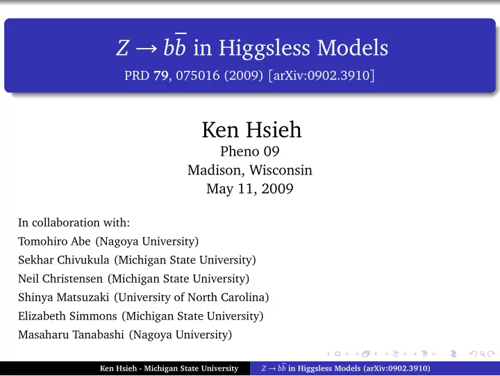
Z → bb in Higgsless Models PRD 79 , 075016 (2009) [ arXiv:0902.3910 ] Ken Hsieh Pheno 09 Madison, Wisconsin May 11, 2009 In collaboration with: Tomohiro Abe (Nagoya University) Sekhar Chivukula (Michigan State University) Neil Christensen (Michigan State University) Shinya Matsuzaki (University of North Carolina) Elizabeth Simmons (Michigan State University) Masaharu Tanabashi (Nagoya University) Ken Hsieh - Michigan State University Z → bb in Higgsless Models (arXiv:0902.3910)

Why Calculate Z → b L b L ? The top quark is special in the SM model. Solutions to the hierarchy problem necessarily involve modifications / additions to the top sector, and the top quark mass sets a scale for flavor hierarchy. Through SU ( 2 ) L , the coupling between Z and b L feels these modifications and the well-measured Z -pole observables (ex: Γ( Z → b L b L ) and A b LR ) serve as strong constraints. In this talk, we elucidate the gaugeless technique of calculating flavor-dependent corrections to Z → b L b L , and apply this technique to the Three-Site Higgsless Model. The reference contains many other ways of understanding the result of this calculation. Ken Hsieh - Michigan State University Z → bb in Higgsless Models (arXiv:0902.3910)

✐ Z → b L b L in the SM The brute-force calculation is straightforward ( m b = 0, m 2 W ≪ m 2 t ): � � � � g Z m 2 ε + ln µ 2 1 ( 4 s 2 W − 4 ) + ( 20 s 2 t = ✐ W − 12 ) 6 192 π 2 v 2 m 2 t g Z m 2 � � � � ε + ln µ 2 1 t ( 7 − 6 s 2 W ) + ( 39 − 30 s 2 = ✐ 6 W ) 192 π 2 v 2 m 2 t � � � � g Z m 2 ε + ln µ 2 1 t ( 2 s 2 W − 3 ) + ( 10 s 2 = ✐ W − 15 ) 6 192 π 2 v 2 m 2 t Ken Hsieh - Michigan State University Z → bb in Higgsless Models (arXiv:0902.3910)

Z → b L b L in the SM The brute-force calculation is straightforward ( m b = 0, m 2 W ≪ m 2 t ): � � � � g Z m 2 ε + ln µ 2 1 ( 4 s 2 W − 4 ) + ( 20 s 2 t = ✐ W − 12 ) 6 192 π 2 v 2 m 2 t g Z m 2 � � � � ε + ln µ 2 1 t ( 7 − 6 s 2 W ) + ( 39 − 30 s 2 = ✐ 6 W ) 192 π 2 v 2 m 2 t � � � � g Z m 2 ε + ln µ 2 1 t ( 2 s 2 W − 3 ) + ( 10 s 2 = ✐ W − 15 ) 6 192 π 2 v 2 m 2 t The result is finite, as expected, because = ✐ g Z m 2 t ⇐ there is no flavor-dependent counter- 16 π 2 v 2 term in the SM. Ken Hsieh - Michigan State University Z → bb in Higgsless Models (arXiv:0902.3910)

The Gaugeless Calculation Barbieri, Beccaria, Ciafaloni, Curi, and Vicere. Phys. Lett. B288 , 95 (1992). Nucl. Phys. B409 , 105 (1993). The key idea: treat Z -boson as external field that couples to J µ θ J µ 3 − s 2 Q .   b   π Z  Z    −→   M Z b For the gaugeless calculation, we compute the coefficient to the op- erator ∂ µ π Z b L γ µ b L and relate to Z → b L b L through a Ward-Takahashi identity     Wavefunction      ∼ M Z +  renormalization       contributions p µ Ken Hsieh - Michigan State University Z → bb in Higgsless Models (arXiv:0902.3910)

✐ π Z → b L b L in the SM This is easier than the Z → b L b L calculation:   = ✐ g Z m 2 t M Z   16 π 2 v 2   p µ   = 0 (No πππ -vertex) M Z     p µ  b  M Z π Z = 0 (No π b L b R -vertex when m b = 0.)   π W   b b t p µ Ken Hsieh - Michigan State University Z → bb in Higgsless Models (arXiv:0902.3910)

π Z → b L b L in the SM This is easier than the Z → b L b L calculation:   = ✐ g Z m 2 t M Z   16 π 2 v 2   p µ   = 0 (No πππ -vertex) M Z     p µ  b  M Z π Z = 0 (No π b L b R -vertex when m b = 0.)   π W   b b t p µ � � = ✐ g Z m 2 There is only one, finite t M Z 16 π 2 v 2 ⇐ diagram in the SM. p µ Ken Hsieh - Michigan State University Z → bb in Higgsless Models (arXiv:0902.3910)

The Gaugeless Limit Barbieri, Beccaria, Ciafaloni, Curi, and Vicere. Phys. Lett. B288 , 95 (1992). Nucl. Phys. B409 , 105 (1993). In the gaugeless limit, we treat the massive Z -boson as an external, clas- sical field that couples to the conserved (before EWSB) current J µ = − M Z ∂ µ π Z + ˆ J µ , J µ = g L ˆ Zbb b L γ µ P L b L + g R Zbb b R γ µ P R b R + ··· . The Ward-Takahashi identity then reads � � � � ∂ x T ˆ J µ ( x ) b ( y ) b ( z ) = M Z T ( � x π Z ( x )) b ( y ) b ( z ) µ �� � � − δ ( x − y ) g L Zbb P L + g R b ( x ) b ( z ) Zbb P R � �� � g L Zbb P R + g R + δ ( x − z ) b ( y ) b ( x ) Zbb P L , Ken Hsieh - Michigan State University Z → bb in Higgsless Models (arXiv:0902.3910)

✐ ✐ ✶ ✶ The Gaugeless Limit - cont. In terms of amputated Green’s functions, we have � � ˆ J µ ( p 1 + p 2 ) b ( p 2 ) b ( p 1 ) ✐ ( p 1 + p 2 ) µ 1PI � � = − ✐ M Z π Z ( p 1 + p 2 ) b ( p 2 ) b ( p 1 ) 1PI − S − 1 � � � � S − 1 bb ( p 1 ) g L Zbb P L + g R + g L Zbb P R + g R bb ( − p 2 ) , Zbb P R Zbb P L Ken Hsieh - Michigan State University Z → bb in Higgsless Models (arXiv:0902.3910)

✐ ✐ ✶ ✶ The Gaugeless Limit - cont. In terms of amputated Green’s functions, we have � � J µ ( p 1 + p 2 ) b ( p 2 ) b ( p 1 ) ˆ ✐ ( p 1 + p 2 ) µ 1PI � � = − ✐ M Z π Z ( p 1 + p 2 ) b ( p 2 ) b ( p 1 ) 1PI − S − 1 � � � � S − 1 bb ( p 1 ) g L Zbb P L + g R + g L Zbb P R + g R bb ( − p 2 ) , Zbb P R Zbb P L We can organize the Ward-Takahashi identity with the Lorentz structure of the Green’s functions Ken Hsieh - Michigan State University Z → bb in Higgsless Models (arXiv:0902.3910)

The Gaugeless Limit - cont. In terms of amputated Green’s functions, we have � � ˆ J µ ( p 1 + p 2 ) b ( p 2 ) b ( p 1 ) ✐ ( p 1 + p 2 ) µ 1PI � � = − ✐ M Z π Z ( p 1 + p 2 ) b ( p 2 ) b ( p 1 ) 1PI � � � � − S − 1 S − 1 g L Zbb P L + g R g L Zbb P R + g R bb ( p 1 ) Zbb P R + Zbb P L bb ( − p 2 ) , We can organize the Ward-Takahashi identity with the Lorentz structure of the Green’s functions  p 1  b  b  p 1 π Z   ✐ ( p / 1 + p / 2 ) J µ = − ✐ M Z ( p / 1 + p / 2 )       p 1 +p 2   b b p 2 p 2 � p γ µ � − 1 � − 1 �� � � � � / 1 g L Zbb P L + g R + g L Zbb P R + g R / 2 , − � p p Zbb P R Zbb P L p � p At tree level, this gives the gauge couplings of the Z -boson. Ken Hsieh - Michigan State University Z → bb in Higgsless Models (arXiv:0902.3910)

The Gaugeless Limit - cont. In terms of amputated Green’s functions, we have � � ˆ J µ ( p 1 + p 2 ) b ( p 2 ) b ( p 1 ) ✐ ( p 1 + p 2 ) µ 1PI � � = − ✐ M Z π Z ( p 1 + p 2 ) b ( p 2 ) b ( p 1 ) 1PI − S − 1 � � � � S − 1 bb ( p 1 ) g L Zbb P L + g R + g L Zbb P R + g R bb ( − p 2 ) , Zbb P R Zbb P L We can organize the Ward-Takahashi identity with the Lorentz structure of the Green’s functions   p 1 b  p 1 b  π Z   J µ ✐ ( p 1 + p 2 ) µ (= 0 ) = − ✐ M Z      p 1 +p 2    b b p 2 p 2 γ 5 γ µ γ 5 � − 1 � − 1 �� � � � � g L Zbb P L + g R g L Zbb P R + g R − Zbb P R + Zbb P L , ✶ ✶ At tree level, this relates the π Z bb coupling to m b . Ken Hsieh - Michigan State University Z → bb in Higgsless Models (arXiv:0902.3910)

✐ ✐ ✐ ✐ ✐ The Ward Identity at Loop-Level The one-loop Zb L b L coupling is given by   p 1 b L , 1-loop   J µ ✐ g = ✐   Zbb   b p 2 γ µ Ken Hsieh - Michigan State University Z → bb in Higgsless Models (arXiv:0902.3910)

✐ ✐ ✐ ✐ ✐ The Ward Identity at Loop-Level The one-loop Zb L b L coupling is given by   p 1 b L , 1-loop �   � J µ ✐ g = ✐ Z L Z L   Zbb b b   b p 2 γ µ Ken Hsieh - Michigan State University Z → bb in Higgsless Models (arXiv:0902.3910)

✐ ✐ ✐ ✐ The Ward Identity at Loop-Level The one-loop Zb L b L coupling is given by   p 1 b L , 1-loop �   � J µ ✐ g = ✐ Z L Z L   Zbb b b   b p 2 γ µ  p 1 b  � − 1 π Z � � � � �� � Z L Z L g L Z L Z L = − ✐ M Z   b − b b b Zbb  p 1 +p 2  � p b p 2 � p Ken Hsieh - Michigan State University Z → bb in Higgsless Models (arXiv:0902.3910)

✐ ✐ The Ward Identity at Loop-Level The one-loop Zb L b L coupling is given by   p 1 b L , 1-loop �   � J µ ✐ g = ✐ Z L Z L   Zbb b b   b p 2 γ µ  p 1 b  � − 1 π Z � � � � �� � Z L Z L g L Z L Z L = − ✐ M Z   b − b b b Zbb  p 1 +p 2  � p b p 2 � p  b  p 1 �� 1 + 1 �� �� 1 + 1 � π Z � L , tree 2 δ Z L 1 − δ Z L 2 δ Z L = − ✐ M Z + ✐ g   b b b Zbb   p 1 +p 2 b p 2 � p Ken Hsieh - Michigan State University Z → bb in Higgsless Models (arXiv:0902.3910)