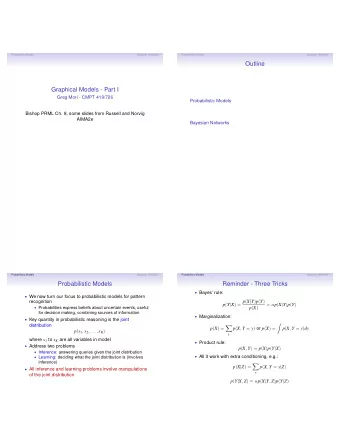
Probabilistic Models Models describe how (a portion of) the world - PowerPoint PPT Presentation

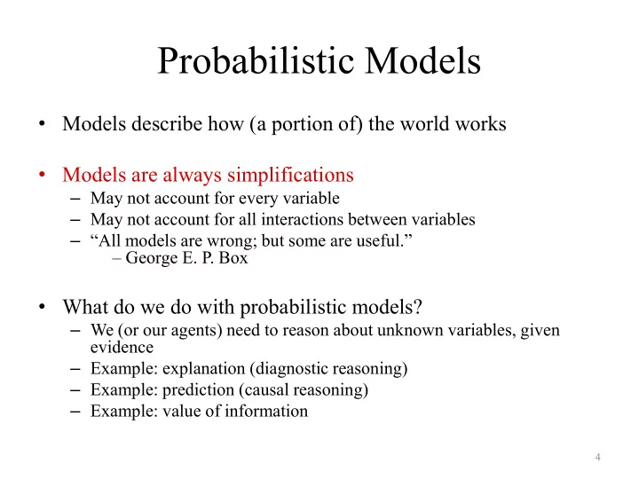
Probabilistic Models • Models describe how (a portion of) the world works • Models are always simplifications – May not account for every variable – May not account for all interactions between variables – “All models are wrong; but some are useful.” – George E. P. Box • What do we do with probabilistic models? – We (or our agents) need to reason about unknown variables, given evidence – Example: explanation (diagnostic reasoning) – Example: prediction (causal reasoning) – Example: value of information 4

Ghostbusters, Revisited • Let’s say we have two distributions: – Prior distribution over ghost location: P(G) • Let’s say this is uniform – Sensor reading model: P(R | G) • Given: we know what our sensors do • R = reading color measured at (1,1) • E.g. P(R = yellow | G=(1,1)) = 0.1 • We can calculate the posterior distribution P(G|r) over ghost locations given a reading using Bayes’ rule: 19

The Chain Rule • Trivial decomposition: • With assumption of conditional independence: • Bayes’ nets / graphical models help us express conditional independence assumptions 5

Model for Ghostbusters � Reminder: ghost is hidden, Joint Distribution sensors are noisy T B G P(T,B,G) � T: Top sensor is red B: Bottom sensor is red +t +b +g 0.16 G: Ghost is in the top � g +t +b 0.16 � Queries: � b +t +g 0.24 P( +g) = ?? � b � g +t 0.04 P( +g | +t) = ?? P( +g | +t, -b) = ?? �� t +b +g 0.04 � t � g +b 0.24 � Problem: joint � t � b +g 0.06 distribution too large / complex � t � b � g 0.06

Ghostbusters Chain Rule � Each sensor depends only P(T,B,G) = P(G) P(T|G) P(B|G) on where the ghost is T B G P(T,B,G) � That means, the two sensors are conditionally independent, given the +t +b +g 0.16 ghost position � g +t +b 0.16 � T: Top square is red � b +t +g 0.24 B: Bottom square is red G: Ghost is in the top � b � g +t 0.04 � Givens: �� t +b +g 0.04 P( +g ) = 0.5 � t � g +b 0.24 P( +t | +g ) = 0.8 P( +t | � g ) = 0.4 � t � b +g 0.06 P( +b | +g ) = 0.4 P( +b | � g ) = 0.8 � t � b � g 0.06

Bayes’ Nets: Big Picture • Two problems with using full joint distribution tables as our probabilistic models: – Unless there are only a few variables, the joint is WAY too big to represent explicitly – Hard to learn (estimate) anything empirically about more than a few variables at a time • Bayes’ nets: a technique for describing complex joint distributions (models) using simple, local distributions (conditional probabilities) – More properly called graphical models – We describe how variables locally interact – Local interactions chain together to give global, indirect interactions – For now, we’ll be vague about how these interactions are specified 11

Example Bayes’ Net: Insurance

Example Bayes’ Net: Car 13

Graphical Model Notation • Nodes: variables (with domains) – Can be assigned (observed) or unassigned (unobserved) • Arcs: interactions – Indicate “direct influence” between variables – Formally: encode conditional independence (more later) • For now: imagine that arrows mean direct causation (in general, they don’t!) 14

Example: Coin Flips • N independent coin flips X 1 X 2 X n • No interactions between variables: absolute independence 15

Example: Traffic • Variables: – R: It rains R – T: There is traffic • Model 1: independence T • Model 2: rain causes traffic • Would an agent using model 2 better? 16

Example: Traffic II • Let’s build a causal graphical model • Variables – T: Traffic – R: It rains – L: Low pressure – D: Roof drips – B: Ballgame – C: Cavity 17

Bayes’ Net Semantics • Let’s formalize the semantics of a Bayes’ net A 1 A n • A set of nodes, one per variable X • A directed, acyclic graph X • A conditional distribution for each node – A collection of distributions over X, one for each combination of parents’ values – CPT: conditional probability table – Description of a noisy “causal” process A Bayes net = Topology (graph) + Local Conditional Probabilities 19

Probabilities in BNs • Bayes’ nets implicitly encode joint distributions – As a product of local conditional distributions – To see what probability a BN gives to a full assignment, multiply all the relevant conditionals together: – Example: • This lets us reconstruct any entry of the full joint • Not every BN can represent every joint distribution – The topology enforces certain conditional independencies 20

Example: Coin Flips X 1 X 2 X n h 0.5 h 0.5 h 0.5 t 0.5 t 0.5 t 0.5 Only distributions whose variables are absolutely independent can be represented by a Bayes’ net with no arcs. 21

Example: Traffic +r 1/4 R � r 3/4 +r +t 3/4 T � t 1/4 � r +t 1/2 � t 1/2 22

Example: Alarm Network E P(E) B P(B) B urglary E arthQk +e 0.002 +b 0.001 � e 0.998 � b 0.999 A larm B E A P(A|B,E) +b +e +a 0.95 J ohn M ary � a +b +e 0.05 calls calls � e +b +a 0.94 � e � a A J P(J|A) A M P(M|A) +b 0.06 � b +e +a 0.29 +a +j 0.9 +a +m 0.7 � b � a � j � m +e 0.71 +a 0.1 +a 0.3 � b � e � a � a +a 0.001 +j 0.05 +m 0.01 � b � e � a � a � j � a � m 0.999 0.95 0.99

Example: Alarm Network P(E) P(B) B urglary E arthQk 0.002 0.001 A larm B E P(A|B,E) +b +e 0.95 J ohn M ary � e +b 0.94 calls calls � b +e 0.29 � b � e A P(J|A) A P(M|A) 0.001 +a 0.9 +a 0.7 � a � a 0.05 0.01

Bayes’ Nets • So far: how a Bayes’ net encodes a joint distribution • Next: how to answer queries about that distribution – Key idea: conditional independence – Main goal: answer queries about conditional independence and influence • After that: how to answer numerical queries (inference) 25

Bayes’ Net Semantics • Let’s formalize the semantics of a Bayes’ net A 1 A n • A set of nodes, one per variable X • A directed, acyclic graph X • A conditional distribution for each node – A collection of distributions over X, one for each combination of parents’ values – CPT: conditional probability table – Description of a noisy “causal” process A Bayes net = Topology (graph) + Local Conditional Probabilities 26

Example: Alarm Network E P(E) B P(B) B urglary E arthqk +e 0.002 +b 0.001 � e 0.998 � b 0.999 A larm B E A P(A|B,E) +b +e +a 0.95 J ohn M ary � a +b +e 0.05 calls calls � e +b +a 0.94 � e � a A J P(J|A) A M P(M|A) +b 0.06 � b +e +a 0.29 +a +j 0.9 +a +m 0.7 � b � a � j � m +e 0.71 +a 0.1 +a 0.3 � b � e � a � a +a 0.001 +j 0.05 +m 0.01 � b � e � a � a � j � a � m 0.999 0.95 0.99

Building the (Entire) Joint • We can take a Bayes’ net and build any entry from the full joint distribution it encodes – Typically, there’s no reason to build ALL of it – We build what we need on the fly • To emphasize: every BN over a domain implicitly defines a joint distribution over that domain, specified by local probabilities and graph structure 28

Size of a Bayes’ Net • How big is a joint distribution over N Boolean variables? 2 N • How big is an N-node net if nodes have up to k parents? O(N * 2 k+1 ) • Both give you the power to calculate • BNs: Huge space savings! • Also easier to elicit local CPTs • Also turns out to be faster to answer queries (coming) 29

Bayes’ Nets So Far • We now know: – What is a Bayes’ net? – What joint distribution does a Bayes’ net encode? • Now: properties of that joint distribution (independence) – Key idea: conditional independence – Last class: assembled BNs using an intuitive notion of conditional independence as causality – Today: formalize these ideas – Main goal: answer queries about conditional independence and influence • Next: how to compute posteriors quickly (inference) 30

Inference by Enumeration • Given unlimited time, inference in BNs is easy • Recipe: – State the marginal probabilities you need – Figure out ALL the atomic probabilities you need – Calculate and combine them • Example: B E A J M 3

Example: Enumeration • In this simple method, we only need the BN to synthesize the joint entries B E A P(+m | +b, +e)? J M 4

• P(+m | +b, +e)? • P(+m, +b, +e) / P(+b, +e) P(+m, +b, +e) = P(+b)P(+e)P(+a|+b,+e)P(+m|+a) + P(+b)P(+e)P(-a|+b,+e)P(+m|-a) Find P(-m, +b, +e) B E Or Find P(+b, +e) A J M

Assume a= true. What is P(B,E)? • P(B,E|+a) =? P(E) P(B) B urglary E arthQk 0.002 0.001 A larm B E P(A|B,E) +b +e 0.95 J ohn M ary � e +b 0.94 calls calls � b +e 0.29 � b � e A P(J|A) A P(M|A) 0.001 +a 0.9 +a 0.7 � a � a 0.05 0.01

Inference by Enumeration? 7

Variable Elimination • Why is inference by enumeration so slow? – You join up the whole joint distribution before you sum out the hidden variables – You end up repeating a lot of work! • Idea: interleave joining and marginalizing! – Called “Variable Elimination” – Still NP-hard, but usually much faster than inference by enumeration • We’ll need some new notation to define VE 8