- What is V aR? - V alue at Risk is the loss, whih is - PowerPoint PPT Presentation
- Qualit y of V alue-at-Risk App ro ximations b y Numerial Solutions of SDEs - Denis T ala y and Ziyu Zheng This w o rk is a joint ollab o ration b et w een the RiskLab and INRIA Sophia Antip olis.
- Qualit y of V alue-at-Risk App ro ximations b y Numeri al Solutions of SDEs - Denis T ala y and Ziyu Zheng This w o rk is a joint ollab o ration b et w een the RiskLab and INRIA Sophia Antip olis. (Institut National de Re her he en Info rmatique et en Automatique) RiskLab Risk Da y 2000 :0 Ω
- What is V aR? - V alue at Risk is the loss, whi h is ex eeded with some given p roba- bilit y α , over a given ho rizon. Mathemati ally , V alue at Risk is the quantile of a random va riable, whi h des rib es the p ossible loss in the future. RiskLab Risk Da y 2000 :1 Ω
- A t ypi al example - A �nan ial ma rk et onsists in N + M + 1 se urities: N sto ks, M b onds and an instantaneous riskless saving a ount. An investment a tivit y is mo delled b y a N + M + 2 dimensional sto hasti di�erential equation, whose solution rep resents the p ri es of N sto ks, the p ri es of M b onds, the saving a ount and the w ealth p ro ess X ( · ) of the trader's p o rtfolio. The V aR ( α ) fo r this investment is the la rgest value su h that P ( X ( T ) − X (0) ≤ V aR ( α )) ≤ α. RiskLab Risk Da y 2000 :2 Ω
- Cal ulation of V aR - The b est w a y to al ulate V aR, of ourse, w ould b e to use an analyti fo rmula. F o r a mo del whose o e� ients a re omplex fun tions o r a high di- mensional mo del, it is imp ossible to al ulate the V aR expli itly . Solution: App ro ximate the V aR b y numeri al metho ds. RiskLab Risk Da y 2000 :3 Ω
- Evaluating existing metho ds - When one ho oses a numeri al metho d fo r V aR al ulation, one has to mak e a tradeo� b et w een a ura y , numeri al ost and generalit y . W e give some omments on some standa rd metho ds. Delta metho d, Delta-gamma metho d and related metho ds a re fast but not very a urate, and they require a simple mo del (whi h de- reases the global a ura y). F ull Monte Ca rlo metho d gives a b etter a ura y , but it requires exa t p ri ing fo rmula (whi h restri ts the hoi e of the mo dels), and is time- onsuming. RiskLab Risk Da y 2000 :4 Ω
- Evaluating existing metho ds ( ont.) - The Grid Monte Ca rlo metho d gives go o d a ura y and an b e applied to general nonlinea r mo dels, but w e re ommend it fo r lo w dimensional p roblems only , fo r a p o rtfolio with a la rge numb er of se urities, the numeri al ost is very exp ensive. RiskLab Risk Da y 2000 :5 Ω
- What is the suitable numeri al metho d to al ulate V aR? - Ma y w e �nd a new metho d, whi h is a urate, an b e applied to general nonlinea r and high dimensional mo dels, and to long-term risk measurement p roblems? W e emphasize that, in the sto hasti mo del as ab ove, The V aR under interest is the quantile of the ma rginal distribution of the solution at ho rizon T to a sto hasti di�erential equation. Thus the p roblem is: �nd a suitable numeri al metho d to app ro ximate su h quantiles. RiskLab Risk Da y 2000 :6 Ω
- The answ er - The Monte Ca rlo metho d. + The Euler s heme. RiskLab Risk Da y 2000 :7 Ω
- What is the Euler s heme? - Let ( X t ) b e a real valued di�usion p ro ess, solution to dX t = b ( X t ) dt + σ ( X t ) dW t , where ( W t ) is a r -dimensional Bro wnian motion. The Euler s heme is a time dis retization of the SDE: pT/n ) T X n ( p +1) T/n = X n pT/n + b ( X n n + σ ( X n pT/n )( W ( p +1) T/n − W pT/n ) . n is the numb er of steps of the dis retization and p = 0 , 1 ,...,n − 1 . X n is a go o d app ro ximation of X T . T RiskLab Risk Da y 2000 :8 Ω
- What is the Monte Ca rlo metho d? - of X n The la w is to o omplex to al ulate expli itly . T of X n W e use N i.i.d. opies to app ro ximate E [ f ( X T )] . T N 1 f ( X n,i � T ) → E [ f ( X T )] , as n,N → ∞ . N i =1 The left hand side an b e easily simulated on a omputer: one simply has to simulate the indep endent Gaussian in rements of the Bro wnian motion. RiskLab Risk Da y 2000 :9 Ω
- The dis retization erro r - Under hyp otheses of unifo rmly hyp o ellipti it y t yp e, X T has a smo oth densit y p X T . Therefo re given a p ositive real 0 < δ < 1 , there exists a quantile ρ ( δ ) su h that P [ X T ≤ ρ ( δ )] = δ. s heme, X n F o r the molli�ed Euler also has a smo oth densit y , thus T quantile ρ n ( δ ) there exists a su h that P [ X n T ≤ ρ n ( δ )] = δ. RiskLab Risk Da y 2000 :10 Ω
- The dis retization erro r ( ont.) - W e have p roved that the dis retization erro r on the quantile satis�es | ρ n ( δ ) − ρ ( δ ) | ≤ C ( T ) q T ( δ ) n, where q T ( δ ) = y ∈ [ ρ ( δ ) − 1 ,ρ ( δ )+1] p X T ( y ) ≃ p X T ( ρ ( δ )) . inf RiskLab Risk Da y 2000 :11 Ω
- The statisti al erro r - X n,i � � W e an so rt the simulated T ,i = 1 ,...,N , and thus get the empi- quantile ρ n ri al N ( δ ) . The lassi al theo ry tell us that the statisti al erro r is of o rder 1 | ρ n ( δ ) − ρ n N ( δ ) | ∼ √ N . q T ( δ ) RiskLab Risk Da y 2000 :12 Ω
- The global erro r of the metho d - Thus the global erro r of the simulated quantile satis�es C ( T ) + C ( T ) E | ρ ( δ ) − ρ n N ( δ ) | ≤ √ q T ( δ ) n. q T ( δ ) N F o r a p ra ti al use, one needs an a urate lo w er b ound of the den- sit y of X T in o rder to ho ose n,N in terms of the desired a ura y . F o r stri tly unifo rm ellipti generato rs, see, e.g., Azen ott. In dege- nerate ase, under restri tive assumption on the drift b , see Kusuok a & Stro o k. RiskLab Risk Da y 2000 :13 Ω
- The ase of high dimension and ma rginal la w - a R d Let ( X t ) b e valued p ro ess, solution to dX t = b ( X t ) dt + σ ( X t ) dW t . y ( X i Denote b t ) the o o rdinate p ro ess of ( X t ) . Supp ose the generato r quantile ρ i ( δ ) of ( X t ) is unifo rmly hyp o ellipti , then there exists a su h that P [ X i T ≤ ρ i ( δ )] = δ. quantile ρ n,i ( δ ) and a of the Euler s heme su h that P [ X n,i ≤ ρ n,i ( δ )] = δ. T RiskLab Risk Da y 2000 :14 Ω
- The ase of a ma rginal la w ( ont.) - W e have p roved | ρ n,i ( δ ) − ρ i ( δ ) | ≤ C ( T ) T ( δ ) n. q i q i p i X T ( y ) ≃ p i X T ( ρ i ( δ )) , T ( δ ) = inf y ∈ [ ρ i ( δ ) − 1 ,ρ i ( δ )+1] where p i is the i -th ma rginal distribution of X T . X T W e re all that the situation here is exa tly the one w e gave in the example fo r the p o rtfolio of N + M + 1 se urities. RiskLab Risk Da y 2000 :15 Ω
- Con lusion - W e on lude b y listing some p rop erties of our numeri al app roa h: 1. A desired a ura y an b e a hieved b y ho osing N and n p rop erly . 2.Our erro r estimates hold fo r hyp o ellipti SDE, whi h is a ommon situation in �nan e. 3. The numeri al ost gro ws only linea rly w.r.t the dimension. Mo reo- ver, the numeri al ost an b e redu ed b y using pa rallel a r hite tures. 4. It an b e applied to long term risk measurement p roblems. RiskLab Risk Da y 2000 :16 Ω
- An appli ation to Mo del Risk measurement - maturities: T O < T Given t w o . y T O The trader w ants to hedge a Europ ean option with maturit written on a dis ount b ond B ( t,T ) . The pa y o� at maturit y is y Φ( B ( T O ,T )) denoted b . The trader uses t w o b onds to hedge the option: the b ond with y T O maturit and the b ond of maturit y T . RiskLab Risk Da y 2000 :17 Ω
- The Heath-Ja rro w-Mo rton mo del - Instantaneous fo rw a rd rate under the sp ot ma rtingale measure: � t � t f ( t,T ∗ ) = f (0 ,T ∗ ) + 0 σ ( s,T ∗ ) σ ∗ ( s,T ∗ ) ds + 0 σ ( s,T ∗ ) dW s , with � T ∗ σ ∗ ( s,T ∗ ) := σ ( s,u ) du. s Dis ount b ond p ri e B ( t,T ) : � T � T σ ∗ ( s,T ) B ( s,T ) dW s , 0 ≤ t ≤ T. B ( t,T ) = 1 − r ( s ) B ( s,T ) ds + t t RiskLab Risk Da y 2000 :18 Ω
- The p o rtfolio - The p o rtfolio V t = H t B ( t,T ) + H O t B ( t,T O ) . Assumption: The p o rtfolio is self-�nan ing, i.e., � t � t 0 H O s dB ( s,T O ) . V t = V 0 + 0 H s dB ( s,T ) + RiskLab Risk Da y 2000 :19 Ω
- The fo rw a rd p ri es of the b ond and of the p o rtfolio - F o rw a rd p ri e of the b ond: B F ( t,T ) := B ( t,T ) B ( t,T O ) . F o rw a rd p ri e of the p o rtfolio: B ( t,T O ) = H t B ( t,T ) + H O t B ( t,T O ) V t V F := . t B ( t,T O ) F rom the self-�nan ing ondition = H t dB F ( t,T ) . dV F t RiskLab Risk Da y 2000 :20 Ω
Recommend
More recommend
Explore More Topics
Stay informed with curated content and fresh updates.

