Weighted SGD for p Regression with Randomized Preconditioning - PowerPoint PPT Presentation
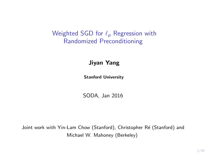
Weighted SGD for p Regression with Randomized Preconditioning Jiyan Yang Stanford University SODA, Jan 2016 Joint work with Yin-Lam Chow (Stanford), Christopher R e (Stanford) and Michael W. Mahoney (Berkeley) 1/29 Outline Overview
Weighted SGD for ℓ p Regression with Randomized Preconditioning Jiyan Yang Stanford University SODA, Jan 2016 Joint work with Yin-Lam Chow (Stanford), Christopher R´ e (Stanford) and Michael W. Mahoney (Berkeley) 1/29
Outline Overview A Perspective of Stochastic Optimization Preliminaries in Randomized Linear Algebra Main Algorithm and Theoretical Results Empirical Results 2/29
Problem formulation Definition Given a matrix A ∈ R n × d , where n ≫ d , a vector b ∈ R n , and a number p ∈ [1 , ∞ ], the constrained overdetermined ℓ p regression problem is min x ∈Z � Ax − b � p . 3/29
Overview low-precision medium-precision high-precision 10 -1 10 -8 SGD pwSGD RLA Efficient, easy, scalable Requires IPM to solve the constrained subproblem Widely used for convex objective Works well for problems with linear structure Asymptotic convergence rate Better worst-case theoretical guarantee Formulated in terms of assumptions Formulated for worst-case inputs pwSGD — Preconditioned weighted SGD ◮ It preserves the simplicity of SGD and the high quality theoretical guarantees of RLA. ◮ It is preferable when a medium-precision, e.g., 10 − 3 is desired. 4/29
Our main algorithm: pwSGD Algorithm 1. Apply RLA techniques to construct a preconditioner and then construct an importance sampling distribution. 2. Apply an SGD-like iterative phase with weighted sampling on the preconditioned system. Properties ◮ The preconditioner and the importance sampling distribution can be done as fast as in O (log n · nnz( A )). ◮ The convergence rate of the SGD phase only depends on the low dimension d , independent of the high dimension n . 5/29
Complexity comparisons solver complexity (general) complexity (sparse) 3 9 69 25 5 2 /ǫ 3 ) 2 8 log 2 ) RLA sampling time ( R ) + O (nnz( A ) log n + ¯ κ 1 d O (nnz( A ) log n + d 8 d /ǫ time ( R ) + nd 2 + O (( nd + poly( d )) log(¯ randomized IPCPM κ 1 d /ǫ )) O ( nd log( d /ǫ )) 13 5 time ( R ) + O (nnz( A ) log n + d 3 ¯ κ 1 /ǫ 2 ) 2 d /ǫ 2 ) 2 log pwSGD O (nnz( A ) log n + d Table: Summary of complexity of several unconstrained ℓ 1 solvers that use randomized linear algebra. Clearly, pwSGD has a uniformly better complexity than that of RLA sampling methods in terms of both d and ǫ , no matter which underlying preconditioning method is used. solver complexity (SRHT) complexity (sparse) � nd log( d /ǫ ) + d 3 log( nd ) /ǫ � � nnz( A ) + d 4 /ǫ 2 � RLA projection O O � nd log n + d 3 log d + d 3 log d /ǫ � � nnz( A ) log n + d 4 + d 3 log d /ǫ � RLA sampling O O � nd log d + d 3 log d + nd log(1 /ǫ ) � � nnz( A ) + d 4 + nd log(1 /ǫ ) � RLA high-precision solvers O O � nd log n + d 3 log d + d 3 log(1 /ǫ ) /ǫ � � nnz( A ) log n + d 4 + d 3 log(1 /ǫ ) /ǫ � pwSGD O O Table: Summary of complexity of several unconstrained ℓ 2 solvers that use randomized linear algebra. When d ≥ 1 /ǫ and n ≥ d 2 /ǫ , pwSGD is asymptotically better than the solvers listed above. 6/29
Outline Overview A Perspective of Stochastic Optimization Preliminaries in Randomized Linear Algebra Main Algorithm and Theoretical Results Empirical Results 7/29
Viewing ℓ p regression as stochastic optimization ( a ) ( b ) x ∈Z � Ax − b � p y ∈Y � Uy − b � p min − − → min − − → min y ∈Y E ξ ∼ P [ H ( y , ξ )] . p p ◮ ( a ) is done by using a different basis U . ◮ ( b ) is true for any sampling distribution { p i } n i =1 over the rows by setting H ( y , ξ ) = | U ξ y − b ξ | p . p ξ 8/29
Solving ℓ p regression via stochastic optimization To solve this stochastic optimization problem, typically one needs to answer the following three questions. ◮ (C 1 ): How to sample: SAA (i.e., draw samples in a batch mode and deal with the subproblem) or SA (i.e., draw a mini-batch of samples in an online fashion and update the weight after extracting useful information)? ◮ (C 2 ): Which probability distribution P (uniform distribution or not) and which basis U (preconditioning or not) to use? ◮ (C 3 ): Which solver to use (e.g., how to solve the subproblem in SAA or how to update the weight in SA)? 9/29
A unified framework for RLA and SGD ℓ p regression naive uniform P fast gradient descent SA vanilla SGD min x � Ax − b � p U = A p online using RLA non-uniform P pwSGD fast n e n l i o gradient descent SA (this presentation) stochastic optimization well-conditioned U min y E ξ ∼ P [ | U ξ y − b ξ | p / p ξ ] b a t c h using RLA exact solution vanilla RLA non-uniform P slow SAA of subproblem sampling algorithm well-conditioned U ( C 1): How to sample? ( C 2): Which U and P to use? ( C 3): How to solve? resulting solver 10/29
Outline Overview A Perspective of Stochastic Optimization Preliminaries in Randomized Linear Algebra Main Algorithm and Theoretical Results Empirical Results 11/29
ℓ p Well-conditioned basis Definition ( ℓ p -norm condition number (Clarkson et al., 2013)) Given a matrix A ∈ R m × n and p ∈ [1 , ∞ ], let σ max � x � 2 =1 � Ax � p and σ min ( A ) = max ( A ) = min � x � 2 =1 � Ax � p . p p Then, we denote by κ p ( A ) the ℓ p -norm condition number of A , defined to be: κ p ( A ) = σ max ( A ) /σ min ( A ) . p p 12/29
Motivation ◮ For ℓ 2 , a perfect preconditioner is the one that transforms A into an orthonormal basis. ◮ However, doing such requires factorizations like QR and SVD of A which is expensive. ◮ Can we do QR on a similar but much smaller matrix? ◮ Idea: we use randomized linear algebra to compute a sketch and perform QR on it. 13/29
An important tool: sketch ◮ Given a matrix A ∈ R n × d , a sketch can be viewed as a compressed representation of A , denoted by Φ A . ◮ The matrix Φ ∈ R r × n preserves the norm of vectors in the range space of A up to small constants. That is, ∀ x ∈ R d . (1 − ǫ ) � Ax � ≤ � Φ Ax � ≤ (1 + ǫ ) � Ax � , ◮ r ≪ n . 14/29
Type of ℓ 2 sketches ◮ Sub-Gaussian sketch e.g., Gaussian transform: Φ A = GA time: O ( nd 2 ), r = O ( d /ǫ 2 ) ◮ Sketch based on randomized orthonormal systems [Tropp, 2011] e.g., Subsampled randomized Hadamard transform (SRHT): Φ A = SDHA time: O ( nd log n ), r = O ( d log( nd ) log( d /ǫ 2 ) /ǫ 2 ) ◮ Sketch based on sparse transform [Clarkson and Woodruff, 2013] e.g., count-sketch like transform (CW): Φ A = RDA time: O ( nnz ( A )), r = ( d 2 + d ) /ǫ 2 ◮ Sampling with approximate leverage scores [Drineas et al., 2012] Leverage scores can be viewed as a measurement of the importance of the rows in the LS fit. e.g., using CW transform to estimate the leverage scores time: t proj + O ( nnz ( A )) log n , r = O ( d log d /ǫ 2 ) Normally, when ǫ is fixed, the required sketching size r only depends on d , independent of n . 15/29
Randomized preconditioners Algorithm 1. Compute a sketch Φ A . 2. Compute the economy QR factorization of Φ A = QR . 3. Return R − 1 . 16/29
Randomized preconditioners (cont’) Analysis ◮ Since A and Φ A are “similar”, AR − 1 ≈ Φ AR − 1 = Q . ◮ Using norm preservation property of the sketch and norm equivalence, we have � AR − 1 x � p ≤ � Φ AR − 1 x � p /σ Φ ≤ r max { 0 , 1 / p − 1 / 2 } · � Φ AR − 1 � 2 · � x � 2 /σ Φ = r max { 0 , 1 / p − 1 / 2 } · � x � 2 /σ Φ , ∀ x ∈ R d , and � AR − 1 x � p ≥ � Φ AR − 1 � p / ( σ Φ κ Φ ) ≥ r min { 0 , 1 / p − 1 / 2 } · � Φ AR − 1 x � 2 / ( σ Φ κ Φ ) = σ Φ r min { 0 , 1 / p − 1 / 2 } · � x � 2 / ( σ Φ κ Φ ) , ∀ x ∈ R d . 17/29
Qualities of preconditioners name running time κ p ( U ) ¯ O ( nd 2 log d + d 3 log d ) O ( d 5 / 2 log 3 / 2 d ) Dense Cauchy [SW11] O ( nd log d + d 3 log d ) O ( d 11 / 2 log 9 / 2 d ) Fast Cauchy [CDM+12] 13 11 O (nnz( A ) + d 7 log 5 d ) Sparse Cauchy [MM12] O ( d 2 log 2 d ) 7 5 O (nnz( A ) + d 3 log d ) 2 log Reciprocal Exponential [WZ13] O ( d 2 d ) Table: Summary of running time and condition number, for several different ℓ 1 conditioning methods. name running time κ p ( U ) ¯ κ p ( U ) √ O ( nd 2 ) sub-Gaussian O (1) O ( d ) √ O ( nd log n + d 3 log d ) SRHT [Tropp11] O (1) O ( d ) √ O (nnz( A ) + d 4 ) Sparse ℓ 2 Embedding [CW12] O (1) O ( d ) Table: Summary of running time and condition number, for several different ℓ 2 conditioning methods. 18/29
Why preconditioning is useful? We can actually show that the convergence rate of using SGD for ℓ p regression problem relies on the ℓ p condition number of the linear system. Using such a randomized preconditioner will drastically reduce the number of iterations needed. 19/29
Outline Overview A Perspective of Stochastic Optimization Preliminaries in Randomized Linear Algebra Main Algorithm and Theoretical Results Empirical Results 20/29
Recommend
More recommend
Explore More Topics
Stay informed with curated content and fresh updates.
