Warm-up Question Describe all the vectors in R 3 which are - - PowerPoint PPT Presentation

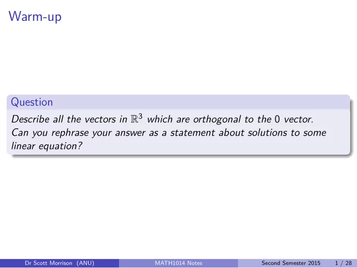
Warm-up

Question

Describe all the vectors in R3 which are orthogonal to the 0 vector. Can you rephrase your answer as a statement about solutions to some linear equation?

Dr Scott Morrison (ANU) MATH1014 Notes Second Semester 2015 1 / 28

Overview

Last week we introduced vectors in Euclidean space and the operations of vector addition, scalar multiplication, dot product, and (for R3) cross product.

Question

How can we use vectors to describe lines and planes in R3? (From Stewart §10.5)

Dr Scott Morrison (ANU) MATH1014 Notes Second Semester 2015 2 / 28

Warm-up

Question

Describe all the vectors in R3 which are orthogonal to the 0 vector. Can you rephrase your answer as a statement about solutions to some linear equation?

Dr Scott Morrison (ANU) MATH1014 Notes Second Semester 2015 3 / 28

Warm-up

Question

Describe all the vectors in R3 which are orthogonal to the 0 vector. Can you rephrase your answer as a statement about solutions to some linear equation? Remember that the statement “v is orthogonal to u" is equivalent to “v · u = 0". This question asks for all the vectors

  

x y z

   such that   

x y z

   ·       = 0.

Using the definition of the dot product, this translates to asking what

  

x y z

   satisfy the equation 0x + 0y + 0z = 0...

...the answer is that all vectors in R3 are orthogonal to the 0 vector. Equivalently, every triple (x, y, z) is a solution to the linear equation 0x + 0y + 0z = 0.

Dr Scott Morrison (ANU) MATH1014 Notes Second Semester 2015 3 / 28

Lines in R2

In the xy-plane the general form of the equation of a line is ax + by = c, where a and b are not both zero. If b = 0 then this equation can be rewritten as y = −(a/b)x + c/b, which has the form y = mx + k. (Here m is the slope of the line and the point (0, k) is its y-intercept.)

Dr Scott Morrison (ANU) MATH1014 Notes Second Semester 2015 4 / 28

Lines in R2

In the xy-plane the general form of the equation of a line is ax + by = c, where a and b are not both zero. If b = 0 then this equation can be rewritten as y = −(a/b)x + c/b, which has the form y = mx + k. (Here m is the slope of the line and the point (0, k) is its y-intercept.)

Example 1

Let L be the line 2x + y = 3. The line has slope m = −2 and the y-intercept is (0, 3).

Dr Scott Morrison (ANU) MATH1014 Notes Second Semester 2015 4 / 28

Alternatively, we could think about this line (y = −2x + 3) as the path traced out by a moving particle. Suppose that the particle is initially at the point (0, 3) at time t = 0. Suppose, too, that its x-coordinate changes at a constant rate of 1 unit per second and its y-coordinate changes as a constant rate of −2 units per second. At t = 1 the particle is at (1, 1). If we assume it’s always been moving this way, then we also know that at t = −2 it was at (−2, 7). In general, we can display the relationship in vector form:

• x

y

• =
• t

−2t + 3

• =
• 3
• + t
• 1

−2

• Dr Scott Morrison (ANU)

MATH1014 Notes Second Semester 2015 5 / 28

Alternatively, we could think about this line (y = −2x + 3) as the path traced out by a moving particle. Suppose that the particle is initially at the point (0, 3) at time t = 0. Suppose, too, that its x-coordinate changes at a constant rate of 1 unit per second and its y-coordinate changes as a constant rate of −2 units per second. At t = 1 the particle is at (1, 1). If we assume it’s always been moving this way, then we also know that at t = −2 it was at (−2, 7). In general, we can display the relationship in vector form:

• x

y

• =
• t

−2t + 3

• =
• 3
• + t
• 1

−2

• What is the significance of the vector v =
• 1

−2

• ?

Dr Scott Morrison (ANU) MATH1014 Notes Second Semester 2015 5 / 28

In this expression, v is a vector parallel to the line L, and is called a direction vector for L. The previous example shows that we can express L in terms of a direction vector and a vector to specific point on L:

Definition

The equation r = r0 + tv is the vector equation of the line L. The variable t is called a parameter. Here, r0 is the vector to a specific point on L; any vector r which satisfies this equation is a vector to some point on L.

Example 2

• x

y

• =
• 3
• + t
• 1

−2

• (1)

is the vector equation of the line L.

Dr Scott Morrison (ANU) MATH1014 Notes Second Semester 2015 6 / 28

If we express the vectors in a vector equation for L in components, we get a collection of equations relating scalars.

Definition

For r =

• x

y

• , r0 =
• x0

y0

• , v =
• a

b

• , the parametric equations of the line

r = r0 + tv are x = x0 + ta y = y0 + tb.

Dr Scott Morrison (ANU) MATH1014 Notes Second Semester 2015 7 / 28

Lines in R3

The definitions of the vector and parametric forms of a line carry over perfectly to R3.

Definition

The vector form of the equation of the line L in R2 or R3 is r = r0 + tv where r0 is a specific point on L and v = 0 is a direction vector for L. The equations corresponding to the components of the vector form of the equation are called parametric equations of L.

Dr Scott Morrison (ANU) MATH1014 Notes Second Semester 2015 8 / 28

Example 3

Let r0 =

  

1 4 −2

   and v =   

1 2 2

  . Then the vector equation of the line L is

r =

  

1 4 −2

   + t   

1 2 2

   .

The line L contains the point (1, 4, −2) and has direction parallel to v =

  

1 2 2

  . By taking different values of t we can find different points on

the line.

Dr Scott Morrison (ANU) MATH1014 Notes Second Semester 2015 9 / 28

Question

For a given line, is the vector equation for the line unique?

Dr Scott Morrison (ANU) MATH1014 Notes Second Semester 2015 10 / 28

Question

For a given line, is the vector equation for the line unique? No, any vector parallel to the direction vector is another direction vector, and each choice of a point on L will give a different r0.

Dr Scott Morrison (ANU) MATH1014 Notes Second Semester 2015 10 / 28

Example 4

The line with parametric equations x = 1 + 2t y = −4t z = −3 + 5t. can also be expressed as x = 3 + 2t y = −4 − 4t z = 2 + 5t.

• r as

x = 1 − 4t y = 8t z = −3 − 10t. Note that a fixed value of t corresponds to three different points on L when plugged into the three different systems.

Dr Scott Morrison (ANU) MATH1014 Notes Second Semester 2015 11 / 28

Symmetric equations of a line

Another way of describing a line L is to eliminate the parameter t from the parametric equations x = x0 + at y = y0 + bt z = z0 + ct If a = 0, b = 0 and c = 0 then we can solve each of the scalar equations for t and obtain x − x0 a = y − y0 b = z − z0 c . These equations are called the symmetric equations of the line L through (x0, y0, z0) parallel to v. The numbers a, b and c are called the direction numbers of L. If, for example a = 0, the equation becomes x = x0, y − y0 b = z − z0 c .

Dr Scott Morrison (ANU) MATH1014 Notes Second Semester 2015 12 / 28

Example 5

Find parametric and symmetric equations for the line through (1, 2, 3) and parallel to 2i + 3j − 4k.

Dr Scott Morrison (ANU) MATH1014 Notes Second Semester 2015 13 / 28

Example 5

Find parametric and symmetric equations for the line through (1, 2, 3) and parallel to 2i + 3j − 4k. The line has the vector parametric form r = i + 2j + 3k + t(2i + 3j − 4k),

• r scalar parametric equations

    

x = 1 + 2t y = 2 + 3t (−∞ < t < ∞). z = 3 − 4t Its symmetric equations are x − 1 2 = y − 2 3 = z − 3 −4 .

Dr Scott Morrison (ANU) MATH1014 Notes Second Semester 2015 13 / 28

Example 6

Determine whether the two lines given by the parametric equations below intersect L1 : x = 1 + 2t, y = 3t, z = 2 − t L2 : x = −1 + s, y = 4 + s, z = 1 + 3s

Dr Scott Morrison (ANU) MATH1014 Notes Second Semester 2015 14 / 28

Example 6

Determine whether the two lines given by the parametric equations below intersect L1 : x = 1 + 2t, y = 3t, z = 2 − t L2 : x = −1 + s, y = 4 + s, z = 1 + 3s If L1 and L2 intersect, there will be values of s and t satisfying 1 + 2t = −1 + s 3t = 4 + s 2 − t = 1 + 3s Solving the first two equations gives s = 14, t = 6, but these values don’t satisfy the third equation. We conclude that the lines L1 and L2 don’t intersect.

Dr Scott Morrison (ANU) MATH1014 Notes Second Semester 2015 14 / 28

Example 6

Determine whether the two lines given by the parametric equations below intersect L1 : x = 1 + 2t, y = 3t, z = 2 − t L2 : x = −1 + s, y = 4 + s, z = 1 + 3s If L1 and L2 intersect, there will be values of s and t satisfying 1 + 2t = −1 + s 3t = 4 + s 2 − t = 1 + 3s Solving the first two equations gives s = 14, t = 6, but these values don’t satisfy the third equation. We conclude that the lines L1 and L2 don’t intersect. In fact, their direction vectors are not proportional, so the lines aren’t parallel, either. They are skew lines.

Dr Scott Morrison (ANU) MATH1014 Notes Second Semester 2015 14 / 28

Planes in R3

We described a line as the set of position vectors expressible as r0 + v, where r0 was a position vector of a point in L and v was any vector parallel to L. We can describe a plane the same way: the set of position vectors expressible as the sum of a position vector to a point in P and an arbitrary vector parallel to P.

x y z r0 r P0 P x y z r0 v

Dr Scott Morrison (ANU) MATH1014 Notes Second Semester 2015 15 / 28

Choose a vector n which is orthogonal to the plane and choose an arbitrary point P0 in the plane.

x y z n r0 r r-r0 P0 P

Dr Scott Morrison (ANU) MATH1014 Notes Second Semester 2015 16 / 28

Choose a vector n which is orthogonal to the plane and choose an arbitrary point P0 in the plane.

x y z n r0 r r-r0 P0 P

How can we use this data to describe all the other points P which lie in the plane?

Dr Scott Morrison (ANU) MATH1014 Notes Second Semester 2015 16 / 28

Choose a vector n which is orthogonal to the plane and choose an arbitrary point P0 in the plane.

x y z n r0 r r-r0 P0 P

How can we use this data to describe all the other points P which lie in the plane? Let r0 and r be the position vectors of P0 and P respectively. The normal vector n is orthogonal to every vector in the plane. In particular n is orthogonal to r − r0 and so we have n·(r − r0) = 0.

Dr Scott Morrison (ANU) MATH1014 Notes Second Semester 2015 16 / 28

This equation n·(r − r0) = 0. (2) can be rewritten as n·r = n·r0. (3) Either of the equations (2) or (3) is called a vector equation of the plane.

Dr Scott Morrison (ANU) MATH1014 Notes Second Semester 2015 17 / 28

Example 7

Find a vector equation for the plane passing through P0 = (0, −2, 3) and normal to the vector n = 4i + 2j − 3k.

Dr Scott Morrison (ANU) MATH1014 Notes Second Semester 2015 18 / 28

Example 7

Find a vector equation for the plane passing through P0 = (0, −2, 3) and normal to the vector n = 4i + 2j − 3k. We have r0 = 0, −2, 3 and n = 4, 2, −3. Thus the vector form is n ·

r − r0 = 0,

• r

Dr Scott Morrison (ANU) MATH1014 Notes Second Semester 2015 18 / 28

Example 7

Find a vector equation for the plane passing through P0 = (0, −2, 3) and normal to the vector n = 4i + 2j − 3k. We have r0 = 0, −2, 3 and n = 4, 2, −3. Thus the vector form is n ·

r − r0 = 0,

• r

(4i + 2j − 3k)· [(x − 0)i + (y + 2)j + (z − 3)k] = 0. Expanding this gives us a scalar equation for the plane...

Dr Scott Morrison (ANU) MATH1014 Notes Second Semester 2015 18 / 28

Given n = A, B, C, r = x, y, z and r0 = x0, y0, z0, the vector equation n·(r − r0) = 0 becomes A, B, C·x − x0, y − y0, z − z0 = 0,

• r

Dr Scott Morrison (ANU) MATH1014 Notes Second Semester 2015 19 / 28

Given n = A, B, C, r = x, y, z and r0 = x0, y0, z0, the vector equation n·(r − r0) = 0 becomes A, B, C·x − x0, y − y0, z − z0 = 0,

• r

A(x − x0) + B(y − y0) + C(z − z0) = 0. (4) Equation (4) is the scalar equation of the plane through P0(x0, y0, z0) with normal vector n = A, B, C.

Dr Scott Morrison (ANU) MATH1014 Notes Second Semester 2015 19 / 28

The equation A(x − x0) + B(y − y0) + C(z − z0) = 0. can be written more simply in standard form Ax + By + Cz + D = 0, where D = −(Ax0 + By0 + Cz0). If D = 0, the plane passes through the origin.

Dr Scott Morrison (ANU) MATH1014 Notes Second Semester 2015 20 / 28

Example 8

Find a scalar equation for the plane passing through P0 = (0, −2, 3) and normal to the vector n = 4i + 2j − 3k.

Dr Scott Morrison (ANU) MATH1014 Notes Second Semester 2015 21 / 28

Example 8

Find a scalar equation for the plane passing through P0 = (0, −2, 3) and normal to the vector n = 4i + 2j − 3k. The vector form is (4i + 2j − 3k)· [(x − 0)i + (y + 2)j + (z − 3)k] = 0, which in scalar form becomes 4(x − 0) + 2(y + 2) − 3(z − 3) = 0 and this is equivalent to 4x + 2y − 3z = −13.

Dr Scott Morrison (ANU) MATH1014 Notes Second Semester 2015 21 / 28

Example 9

Find a scalar equation of the plane containing the points P = (1, 1, 2), Q = (0, 2, 3), R = (−1, −1, −4).

Dr Scott Morrison (ANU) MATH1014 Notes Second Semester 2015 22 / 28

Example 9

Find a scalar equation of the plane containing the points P = (1, 1, 2), Q = (0, 2, 3), R = (−1, −1, −4). First, we should find a normal vector n to the plane, and there are several ways to do this.

Dr Scott Morrison (ANU) MATH1014 Notes Second Semester 2015 22 / 28

Example 9

Find a scalar equation of the plane containing the points P = (1, 1, 2), Q = (0, 2, 3), R = (−1, −1, −4). First, we should find a normal vector n to the plane, and there are several ways to do this. The vector n = n1i + n2j + n3k will be perpendicular to − → PQ = −i + j + k and − → PR = −2i − 2j − 6k. Therefore, we can solve a system of linear equations: 0 = n · (−i + j + k) = −n1 + n2 + n3 0 = n · (−2i − 2j − 6k) = −2n1 − 2n2 − 6n3. One solution to this system is n = −i − 2j + k, so this is an example of a normal vector to the plane containing the 3 given points.

Dr Scott Morrison (ANU) MATH1014 Notes Second Semester 2015 22 / 28

We can use this normal vector n = −i − 2j + k, together with any one of the given points to write the equation of the plane. Using Q =

  

2 3

  , the

equation is −(x − 0) − 2(y − 2) + 1(z − 3) = 0, which simplifies to x + 2y − z = 1.

Dr Scott Morrison (ANU) MATH1014 Notes Second Semester 2015 23 / 28

The first step in this example was finding the normal vector n, but in fact, there’s another way to do this. Recall that in R3 only, there is a product of two vectors called a cross

• product. The cross product of a and b is a vector denoted a×b which is
• rthogonal to both a and b. If we have two nonzero vectors a and b

parallel to our plane, then n = a×b is a normal vector.

Dr Scott Morrison (ANU) MATH1014 Notes Second Semester 2015 24 / 28

Example 10

Consider the two planes x − y + z = −1 and 2x + y + 3z = 4. Explain why the planes above are not parallel and find a direction vector for the line of intersection.

Dr Scott Morrison (ANU) MATH1014 Notes Second Semester 2015 25 / 28

Example 10

Consider the two planes x − y + z = −1 and 2x + y + 3z = 4. Explain why the planes above are not parallel and find a direction vector for the line of intersection. Two planes are parallel if and only if their normal vectors are parallel. Normal vectors for the two planes above are for example n1 = i − j + k and n2 = 2i + j + 3k

• respectively. These vectors are not parallel, so the planes can’t be parallel

and must intersect. A vector v parallel to the line of intersection is a vector which is orthogonal to both the normal vectors above. We can find such a vector by calculating the cross product of the normal vectors: v =

• i

j k 1 −1 1 2 1 3

• = −4i − j + 3k.

Dr Scott Morrison (ANU) MATH1014 Notes Second Semester 2015 25 / 28

Example 11

Find the line through the origin and parallel to the line of intersection of the two planes x + 2y − z = 2 and 2x − y + 4z = 5.

Dr Scott Morrison (ANU) MATH1014 Notes Second Semester 2015 26 / 28

Example 11

Find the line through the origin and parallel to the line of intersection of the two planes x + 2y − z = 2 and 2x − y + 4z = 5. The planes have respective normals n1 = i + 2j − k and n2 = 2i − j + 4k. A direction vector for their line of intersection is given by v = n1×n2 = 7i − 6j − 5k. A vector parametric equation of the line is r = t(7i − 6j − 5k), since the line passes through the origin.

Dr Scott Morrison (ANU) MATH1014 Notes Second Semester 2015 26 / 28

Parametric equations for this line are, for example, x = 7t y = −6t z = −5t and the corresponding symmetric equations are x 7 = y −6 = z −5.

Dr Scott Morrison (ANU) MATH1014 Notes Second Semester 2015 27 / 28

Recommended exercises for review

Stewart §10.5: 1, 3, 15, 19, 25, 29, 35

Dr Scott Morrison (ANU) MATH1014 Notes Second Semester 2015 28 / 28