Volume Rendering Reference Material The slides have used/adapted - PowerPoint PPT Presentation
Volume Rendering Reference Material The slides have used/adapted material from the following references: 1. Advanced Animation and Rendering Techniques by Watt and Watt 2. Slides by Prof Parag Chaudhuri of Course CS 775 on Volume Graphics 3.
Volume Rendering
Reference Material The slides have used/adapted material from the following references: 1. Advanced Animation and Rendering Techniques by Watt and Watt 2. Slides by Prof Parag Chaudhuri of Course CS 775 on Volume Graphics 3. Slides by Prof Bong Soo Sohn of Lecture on Direct Volume Rendering 4. Lecture Slides on Contouring by Prof Tao Ju (Course CSE554)
Volume Rendering Conventional Rendering I x y ( , ) Bicubic Parametric Patches 2D Image Polygons 3D Structured Objects
Volume Rendering V x y z ( , , ) Scalar Field:
Volume Rendering
Volume Rendering V x y z ( , , ) 2D Scalar Image Structured 3D 3D Scalar Field Model V x y z ( , , ) 3D Scalar Field
Volume Rendering • Polylines (2D) or meshes (3D) that tile the object boundary • Smoother appearance • Less storage (no interior pieces) Binary picture Boundary mesh
Volume Rendering • Creates a binary picture from a grayscale image • How to create a smooth boundary at the threshold? • Such boundary is known as an iso-contour (or iso-curve, iso-surface, etc.) Digital image Binary picture Boundary curve
Volume Rendering • Iso-contour: set of points at a particular function value • Given a continuous function f defined on every point in the space • An iso-contour is all points where f evaluates to be some value c (called the iso-value) • Iso-curves: iso-contours of 2D functions {{ x , y } | f ( x , y ) c } = 2 2 f ( x , y ) x y = + f ( x , y ) 1 =
Volume Rendering • Iso-surfaces: iso-contours of 3D functions {{ x , y , z } | f ( x , y , z ) c } = 2 2 2 f ( x , y , z ) x y z = + + f ( x , y , z ) 1 =
Volume Rendering • Closed • With a well-defined inside and outside • Inside: points above the iso- value • Outside: points below the iso- value • Orthogonal to gradient directions • In general, a manifold Black curves: iso-contours Red arrows: gradient directions Green dots: critical points
Volume Rendering • Input • A grid where each grid Grid point point (pixel or voxel) has a (pixel) Grid edge value (color) Grid cell • An iso-value (threshold) • Output • A closed, manifold, non- intersecting polyline (2D) or mesh (3D) that Iso-value = separates grid points above or below the iso- value
Volume Rendering • For each grid cell with a sign change • Create one vertex on each grid edge with a sign change • Connect vertices by lines
Volume Rendering • Creating vertices • Assuming the underlying, continuous function is linear on the grid edge • Linearly interpolate the positions of the two grid points f1 f t 0 = f f f ! + 0 1 t 1-t x x t ( x x ) = + ! 0 1 0 {x1,y1 } 0 y y t ( y y ) {x0,y0} = + ! {x,y} 0 1 0 - f0
Volume Rendering • Connecting vertices by lines 1 1 2 • Lines shouldn’t intersect 4 “ 0 0 0 1 ” • Each vertex is used once 3 {{2,4}} • So that the polyline is a closed manifold 3 4 2 • Two approaches • Do a walk around the grid cell • Connect consecutive pair of vertices “ 0 0 1 1 ” • Or, using a pre-computed look-up {{3,4}} table • 2^4=16 entries • For each sign combination at the 4 corners, it stores the indices of the “ 1 0 0 1 ” grid edges whose vertices make up {{1,3},{2,4}} the lines.
Volume Rendering
Volume Rendering
Volume Rendering Marching Square • Select a cell 1 1 3 0 2 C D D C 1 • Calculate inside/outside state of each vertex E F E C 3 E G D , 2 • Determine which edge is intersected , C H E 1 • Move to next cell till all cells are
Volume Rendering 1 1 3 No intersection 0 2 ? @ @ ? 1 Contour intersects 2 edges A B A ? (no ambiguity) 3 A C @ , 2 Contour intersects 2 edges (no ambiguity) , ? D A 1 Contour intersects 2 edges (ambiguity)
Volume Rendering 1 1 3 0 No intersection 2 ? @ @ ? 1 Contour intersects 2 edges A B A ? 3 (no ambiguity) A C @ , 2 Contour intersects 2 edges (no ambiguity) , ? D A 1 Contour intersects 2 edges (ambiguity)
Volume Rendering 0 1 1 3 2 No intersection ? @ @ ? 1 Contour intersects 2 edges A B A ? 3 (no ambiguity) A C @ , 2 Contour intersects 2 edges (no ambiguity) , ? D A 1 Contour intersects 2 edges (ambiguity)
Volume Rendering 1 1 3 0 No intersection 2 ? @ @ ? 1 Contour intersects 2 edges A B A ? 3 (no ambiguity) A C @ , 2 Contour intersects 2 edges (no ambiguity) , ? D A 1 Contour intersects 2 edges (ambiguity)
Volume Rendering
Volume Rendering Current cube Previously dealt with New vertex Direction of march
Volume Rendering • To calculate surface normal, we need to determine gradient vector, g (derivative of the density function). • To estimate the gradient vector at the surface of interest, we first estimate the gradient vectors at the vertices and interpolate the gradient at the intersection. • The gradient at cube vertex (i , j, k), is estimated using central differences along the three coordinate axes by: D (i, j, k) is the density at pixel (i, j) in slice k. ! x, ! y, ! z are lengths of the cube edges
Volume Rendering
Volume Rendering
Volume Rendering V x y z ( , , ) = k y j + 1 = y j = Polygon structure generated by “ skimming ”
Volume Rendering
Volume Rendering • scalar field – like temperature in room at each (x,y,z) • many applications – medical (MRI, CT, PET) – geophysical – fluid dynamics
Volume Rendering
Direct Volume Rendering • 3D volume data are represented by a finite number of cross sectional slices (hence a 3D raster) • On each volume element (voxel), stores a data value (if it uses only a single bit, then it is a binary data set. Normally, we see a gray value of 8 to 16 bits on each voxel.) N x 2D arrayes = 3D array
Direct Volume Rendering Based on the idea of ray tracing • Trace from eat each pixel as a ray into object space • Compute color value along the ray • Assign the value to the pixel
Direct Volume Rendering • Maps voxel data values to optical properties Voxel Data Optical Properties • Density • Color • Temperature • Opacity • Color/opacity map • Emphasize or classify features of interest in the data • Piecewise linear functions, Look-up tables, 1D, 2D • GPU – simple shader functions, texture lookup tables
Direct Volume Rendering • Stepping through the volume: a ray is cast into the volume, sampling the volume at certain intervals • The sampling intervals are usually equi-distant, but don’t have to be (e.g. importance sampling) • At each sampling location, a sample is interpolated / reconstructed from the grid voxels • popular filters are: nearest neighbor (box), trilinear (tent), Gaussian, cubic spline • Along the ray - what are we looking for?
Volume Rendering Light Source Eye Point R ! t 1 Density: t 2 t D x t ( ( ), ( ), ( )) y t z t D t ( ) = Illumination: I x t ( ( ), ( ), ( )) y t z t I t ( ) = D x y z ( , , ) Light scattered along R in direction of eye from point at t: I t D t P ( ) ( ) cos !
Volume Rendering t " % Attenuation of light scattered from point t: exp ) D s ds ( ) ! ( $ ' $ ' # & t 1 Summing the intensity of light arriving at the eye along R from all of the elements: t t ( , " % 2 * * B / exp D s ds ( ) I t D t P ( ) ( ) cos dt = ! 0 / 1 $ ' ) - * * $ ' # & t + t . 1 1
Volume Rendering V x y z ( , , ) Image Plane C R ( ) R C R k ( , ) ( , ) R k !
Volume Rendering Determining the color of a voxel: C i j k ( , , ) Calculated using the Phong model, assuming that the normal is given by the gradient: ! V x y z ( , , ) i j k Determining the opacity: ! ( , , ) i j k ! ( X ) ! f 3 ! f 2 ! f 4 ! f 1 V X ( ) f 1 f 2 f 3 f 4
Volume Rendering C R k ( , ) kth voxel along R ( , ) R k ! C out C in C C ( 1 ( , )) R k C R k ( , ) ( , ) R k = ! " + " out in Opacity Transparency Term Term K K " % C R ( ) C R k ( , ) ( , ) R k ( 1 ( , )) R i ) ( = * ! * # & $ ' k 0 i k 1 = = +
Volume Rendering
Volume Rendering Intensity Max Average Accumulate First Depth
Volume Rendering Intensity First Depth
Volume Rendering Intensity Average Depth • Average : produces basically an X-ray picture
Volume Rendering Intensity Max Depth • Max : Maximum Intensity Projection used for Magnetic Resonance Angiogram
Volume Rendering Intensity Accumulate Depth • Accumulate opacity while compositing colors : make transparent layers visible! Levoy ‘88
Volume Rendering color opacity 1.0 object (color, opacity)
Volume Rendering volumetric compositing color opacity 1.0 object (color, opacity)
Volume Rendering Interpolation volumetric compositing kernel color opacity 1.0 object (color, opacity)
Volume Rendering Interpolation volumetric compositing kernel color c = c s ! s(1 - ! ) + c opacity ! = ! s (1 - ! ) + ! 1.0 object (color, opacity)
Recommend
More recommend
Explore More Topics
Stay informed with curated content and fresh updates.
