Very simple control We assume that everything is linear This - PowerPoint PPT Presentation
Very simple control We assume that everything is linear This creates huge mathematical simplifications Linear system: accepts a signal x(t) produces a signal y(t)=K x(t) AND K (x(t) + y(t)) = K x(t) +K y(t) K (a x(t))=
Very simple control
We assume that everything is linear • This creates huge mathematical simplifications • Linear system: • accepts a signal x(t) • produces a signal y(t)=K x(t) • AND • K (x(t) + y(t)) = K x(t) +K y(t) • K (a x(t))= a K x(t) • (notice this means K 0 = 0) K stands for a linear operator, so that (for example) we could have K x(t) = a x(t) or K x(t) = dx/dt
In fact, study only the response to a step • You can approximate any function with a lot of steps • Step is u(t) • this is 0 for t<=0, 1 otherwise • so u(t)-u(t+dt) is a bar • Approximate f(t) by X f ( i ∆ t )( u ( i ∆ t ) − u ( i ∆ t + ∆ t )) i • ex: simplify this expression • ex: we know K u(t) - what is K f(t)?
Ideas: plant/process, control • Plant/process is the thing we wish to control • assume: 1 input, 1 output, linear • for simple examples, I’ll write out the form of the plant • but very often, it isn’t known exactly • System Identification • Control: • supply the plant with the input needed to produce the output you want • Q: why is this hard? • A1: Plant may not be exactly known • A2: Plant may have dynamics • A3: Desired output may change
The very simplest control • Plant: K x(t) = c x(t) • here c is a known constant • We’d like the output to be 1 • feed plant with 1/c • and go home early • Example of open loop control • compute a fixed input and supply to plant • whatever the plant • Advantages: • simple, sometimes works • Disadvantages: • what if your model is wrong?
History of feedback Watt’s flyball governor, C19 These were still in use in late C20!
Closed loop control • Derive an input to the plant from • setpoint (where you want the output to be) • current plant output • The form we will discuss is: Controller Plant Setpoint i(t) + c(t) o(t) G H -
We have c(t)=G (i(t)-o(t)) o(t)=H c(t) so which you should remember o(t)+H G o(t)=H G i(t) Controller Plant i(t) + c(t) o(t) G H -
Simple, worrying example • H c(t) = a c(t) • G x(t) = b x(t) • o(t)+ab o(t)=ab i(t) • Now imagine that i(t) is a step function • for t>0 we have • o(t)= ab/(1+ab) • which isn’t what we wanted • (remember, i(t) is the output value we want) • steady state error is lim t->infinity (o(t)-i(t))
Fix with integral term • Idea: • if (i(t)-o(t)) is not zero, there should be some control input • magnitude increases until it is zero • Z t Gx ( t ) = bx ( t ) + c x ( s ) ds 0 i(t) + c(t) o(t) G H -
Fixing with integral term Z t Z t o ( t ) + abo ( t ) + ac o ( s ) ds = abi ( t ) + ac x ( s ) ds 0 0 Differentiate (1 + ab ) do ( t ) + aco ( t ) = abdi ( t ) + aci ( t ) dt dt BUT we’re interested in t>0, and i(t) is a step at 0 (1 + ab ) do ( t ) + aco ( t ) = aci ( t ) dt
Fixing with integral term (1 + ab ) do ( t ) + aco ( t ) = ac dt Assume that do/dt -> 0 as t-> infinity (we’ll see it does in a moment) o ( t ) = 1 For large t, which is what we wanted
Fixing with integral term do ac dt + 1 + abo ( t ) = 1 o (0) = 0 − ac 1+ ab t ) o ( t ) = (1 − e
Example • is it a good idea to get a faster response by making c bigger?
A more interesting plant Force V(t) F(t) Z t F ( s ) Car v ( t ) = v (0) + m dt 0 • Apply a force to the car to control its velocity • eg braking Input Output Z t F ( s ) v ( t ) = m dt 0
Proportional control Gx ( t ) = bx ( t ) o(t)+H G o(t)=H G i(t) o ( t ) + H [ bo ( t )] = H [ bi ( t )] Z t Z t o ( t ) + b o ( s ) ds = b i ( s ) ds m m 0 0 do dt + b mo ( t ) = b Recall that t>0, i(t)=1 m
Notice do dt + b mo ( t ) = b m − bt m ) o ( t ) = (1 − e • steady state error is now zero • larger b/m -> faster response • BUT larger forces applied to car • (obvious) b/m <0 -> unstable behavior • Example
Examples Small b/m -> low rise time 2 output proportional term 1.5 demand 1 0.5 0 -0.5 -1 -1.5 -2 0 1 2 3 4 5 6 7 8 9 10
Examples Bigger b/m -> faster rise time 2 output proportional term 1.5 demand 1 0.5 0 -0.5 -1 -1.5 -2 0 1 2 3 4 5 6 7 8 9 10
Examples Very big b/m -> fastrise time 2 output proportional term 1.5 demand 1 0.5 0 -0.5 -1 -1.5 -2 0 1 2 3 4 5 6 7 8 9 10
Examples Gigantic b/m -> integrator panics 2 output proportional term 1.5 demand 1 0.5 0 -0.5 -1 -1.5 -2 0 1 2 3 4 5 6 7 8 9 10
Examples Gigantic b/m, smarter integrator-> very fast rise time 2 output proportional term 1.5 demand 1 0.5 0 -0.5 -1 -1.5 -2 0 1 2 3 4 5 6 7 8 9 10
Proportional - Integral (PI) control Z t Gx ( t ) = bx ( t ) + c x ( s ) ds o(t)+H G o(t)=H G i(t) 0 Z t Z t � � o ( t ) + H bo ( t ) + c o ( s ) ds = H bi ( t ) + c i ( s ) ds 0 0 Z t Z u Z t Z u � � o ( t ) + 1 = 1 bo ( u ) + c o ( s ) ds bi ( u ) + c i ( s ) ds m m 0 0 0 0 d 2 o dt 2 + b do dt + c mo ( t ) = c (recall t>0, i(t)=1) m m
d 2 o dt 2 + b do dt + c mo ( t ) = c m m Assume derivatives ->0 as t-> infinity (we’ll see they do) then o(t) = 1 for very large t, which is what we wanted A 1 e zt + A 2 t + A 3 ✓ ◆ A 1 z 2 + b c + A 2 t c m = c c e zt m [ A 1 z + A 2 ] + A 1 m + A 3 m m A 2 = 0 z 2 + b mz + c A 3 = 1 m = 0 A 1 = − 1 (o(0)=0)
z 2 + b mz + c m = 0 (1 − e zt ) Where " # r b 2 z = 1 − b m 2 − 4 c m ± 2 m Cases: Stability: b^2-4cm >0 (two real roots; sum of exponentials) -b/m >0 - soln GROWS with time, otherwise OK b^2-4cm=0 (two copies of the same root - this is known as critical damping) b^2-4cm<0 (sinusoid with exponential amplitude)
Careful with b " # r • small c b 2 z = 1 − b m 2 − 4 c m ± m 2 c = ✏ b 2 m • gives roots that are like − b m (1 − ✏ 4) Might be quite fast − b ✏ rather a lot slower m 4
Examples PI control m=1, b=10, c=25 10 output integral term 9 proportional term demand 8 7 6 5 4 3 2 1 0 0 1 2 3 4 5 6 7 8 9 10
Examples PI control m=1, b=10, c=1 10 output integral term 9 proportional term 8 7 6 5 4 3 2 1 0 0 1 2 3 4 5 6 7 8 9 10
Examples PI control m=1, b=10, c=300 20 output integral term 15 proportional term 10 5 0 -5 -10 -15 -20 0 1 2 3 4 5 6 7 8 9 10
Examples PI control m=1, b=10, c=300 step waveform 2 demand output 1.5 1 0.5 0 -0.5 -1 -1.5 -2 0 1 2 3 4 5 6 7 8 9 10
Examples PI control m=1, b=1, c=300 20 output integral term 15 proportional term 10 5 0 -5 -10 -15 -20 0 1 2 3 4 5 6 7 8 9 10
Examples PI control m=1, b=1, c=300 step waveform 2 demand output 1.5 1 0.5 0 -0.5 -1 -1.5 -2 0 1 2 3 4 5 6 7 8 9 10
More on quadratic equations! Damping ⇣ ⌘ z 2 + 2 ζω z + ω 2 = 0 p 1 − ζ 2 z = − ω ζ ± i Natural frequency Critical damping occurs when there is a double root equivalently when zeta=1 zeta <1 underdamped (soln. wobbles) zeta>1 overdamped (slow rise time)
More on quadratic equations! Damping ⇣ ⌘ z 2 + 2 ζω z + ω 2 = 0 p 1 − ζ 2 z = − ω ζ ± i Natural frequency Our equation r c b ζ = 1 z 2 + b mz + c ω = m = 0 √ cm 2 m b = 2 √ cm Critical damping:
Examples PI control critical damping m=1, b=20, c=100 20 output integral term 15 proportional term 10 5 0 -5 -10 -15 -20 0 1 2 3 4 5 6 7 8 9 10
A derivative term • Issue: • may be hard to get fast rise time • big m requires big b for critical damping • this may be because we are feeding back the current error • Idea: • predict future error • this is equivalent to feeding back some fraction of the derivative
The most important slide • A very high fraction of all controllers in the real world are: Z t dx Gx ( t ) = K i x ( u ) du + K p x ( t ) + K d dt 0 • PID controller
A more interesting plant Force V(t) F(t) Z t F ( s ) Car v ( t ) = v (0) + m dt 0 • Apply a force to the car to control its velocity • eg braking Input Output Z t F ( s ) v ( t ) = m dt 0
Example PID control critical damping m=1, kp=20, ki=100, kd=0 20 output integral term 18 proportional term demand 16 14 12 10 8 6 4 2 0 0 0.1 0.2 0.3 0.4 0.5 0.6 0.7 0.8 0.9 1
Proportional-Integral-Derivative (PID) control Thrash through math of PI slide, and end up with: d 2 o K p do K i K i o = dt 2 + dt + m + K d m + K d m + K d d 2 o dt 2 + b do dt + c mo ( t ) = c Compare to: m m Kd makes the mass look smaller!
Examples PID control critical damping m=100, kp=20, ki=100, kd=0 20 output integral term 18 proportional term demand 16 14 12 10 8 6 4 2 0 0 0.1 0.2 0.3 0.4 0.5 0.6 0.7 0.8 0.9 1
Examples PID control critical damping m=100, kp=20, ki=100, kd=-99 20 output integral term 18 proportional term demand 16 14 12 10 8 6 4 2 0 0 0.1 0.2 0.3 0.4 0.5 0.6 0.7 0.8 0.9 1
Kd Ki Kp
Yet more interesting plant damper Mass F(t) Apply a force to the mass, want to control its position. spring x(t) md 2 x dt 2 + bdx dt + kx = F
Recommend
More recommend
Explore More Topics
Stay informed with curated content and fresh updates.
