Topic # 3 Second-order Systems Reference textbook : Control - PowerPoint PPT Presentation
ME 779 Control Systems Topic # 3 Second-order Systems Reference textbook : Control Systems, Dhanesh N. Manik, Cengage Publishing, 2012 1 Control Systems: Second-order Systems Learning Objectives Differential equations Normalized form
ME 779 Control Systems Topic # 3 Second-order Systems Reference textbook : Control Systems, Dhanesh N. Manik, Cengage Publishing, 2012 1
Control Systems: Second-order Systems Learning Objectives • Differential equations • Normalized form of differential equations • System transfer function • Pole-zero map • Overdamping • Critical damping • Underdamping • Undamped • Impulse, step, sinusoidal repsonse • Frequency response: magnitude and phase 2
Control Systems: Second-order Systems Differential equation m y c y k y K x ( t ) y(t) response Mass, m (kg) Damping coefficient, c (N-s/m) Stiffness, k (N/m) K static sensitivity x(t) input 3
Control Systems: Second-order Systems Differential equation: Normalized form c k Kx ( t ) By dividing throughout by m y y y m m m Undamped natural frequency, rad/s k n m c Damping factor 2 km Kx t ( ) 2 y 2 y y n n m 4
Control Systems: Second-order Systems System transfer function Kx t ( ) 2 y 2 y y n n m Y s ( ) K 2 2 X s ( ) m s 2 s n n 5
Control Systems: Second-order Systems Classification of damping factors Damping Type Property factor 1 Overdamped Exponential decay 1 Critically damped Exponential decay 1 Underdamped Oscillatory decay Undamped Oscillatory 0 6
Control Systems: Second-order Systems Pole-zero map Y s ( ) K ζ >1 overdamped 2 2 X s ( ) m s 2 s n n Poles 2 2 2 2 4 n n n s 1,2 2 2 s 1 1,2 n 7
Control Systems: Second-order Systems Y s ( ) K Pole-zero map ζ =1 critically damped 2 2 X s ( ) m s 2 s n n Poles 2 2 2 2 4 n n n s 1,2 2 s 1,2 n 8
Control Systems: Second-order Systems Y s ( ) K Pole-zero map ζ <1 underdamped 2 2 X s ( ) m s 2 s n n 2 2 2 j 4 2 n n n s 1,2 2 Damped natural 2 1 frequency d n s j tan 1,2 n d 2 1 Poles 9
Control Systems: Second-order Systems Pole-zero map Y s ( ) K ζ =0 undamped 2 2 X s ( ) m s j ω j n x n s-plane j s 1,2 n Poles σ j x n 10
Control Systems: Second-order Systems Overdamped case (ζ>1) Impulse response K 2 Differential equation y 2 y y x ( ) t n n i m Kx 1 i Y s ( ) Laplacian of the output 2 2 m s 2 s n n Kx 1 1 i 2 2 2 2 m 1 ( s 1) ( s 1 n n n n n 11
Control Systems: Second-order Systems Impulse response Overdamped case (ζ>1) Kx 1 1 i Y s ( ) 2 2 2 2 m 1 ( s 1) ( s 1 n n n n n Kx n t 2 i y t ( ) e sinh 1 t n 2 m 1 n Time-domain response 12
Control Systems: Second-order Systems Impulse response Critically damped case ( ζ=1 ) Kx 1 Kx 1 i i Y s ( ) 2 2 2 m s 2 s m s n n n Kx n t i y t ( ) te n m n 13
Control Systems: Second-order Systems Impulse response Undamped case ( ζ<1 ) Poles s j 12 n d Laplace output Kx 1 i Y s ( ) m ( s j )( s j ) n d n d Kx Time-domain n t i y t ( ) e sin t output d m d 14
Control Systems: Second-order Systems Impulse response Undamped case ( ζ<1 ) Kx n t i y t ( ) e sin t d m d K n t Impulse response h t ( ) e sin t function d m d t K y t ( ) e sin F t ( ) d n d m d 0 Duhamel’s integral 15
Control Systems: Second-order Systems Impulse response 16
Control Systems: Second-order Systems Step response Overdamped case (ζ>1) Laplace of the Kx 1 1 i output Y s ( ) m s 2 2 s 1) s 1 n n n n Kx n t 2 2 i y t ( ) 1 e cosh 1 t sinh 1 t n n 2 m 2 1 n Time-domain output 17
Control Systems: Second-order Systems Step response Underdamped case ( ζ<1 ) Kx 1 1 i Laplace of the Y s ( ) output m s ( s j )( s j ) n d n d Kx n t i y t ( ) 1 e cos t sin t d d 2 m 2 1 n Time-domain of the output 18
Control Systems: Second-order Systems Step response Underdamped case ( ζ<1 ) 19
Control Systems: Second-order Systems Step response Underdamped case ( ζ<1 ) n t j ω Kx e i y t ( ) 1 sin( t ) x d 2 m 2 1 n s-plane 2 1 1 tan σ tan 2 1 x 20
Control Systems: Second-order Systems Control Systems: Second-order Systems Step response Underdamped case ( ζ<1 ) 2 t y t m ( ) e n r r n 1 1 sin( t ) d r Kx 2 1 i t Rise time r d 21
Control Systems: Second-order Systems Control Systems: Second-order Systems Step response Underdamped case ( ζ<1 ) t Peak time p d Kx 2 1 Peak response i y t ( ) 1 e p 2 m n 22
Control Systems: Second-order Systems Control Systems: Second-order Systems Step response Underdamped case ( ζ<1 ) Percentage overshoot M p y t ( ) y 2 p 1 M e % p y 23
Control Systems: Second-order Systems Control Systems: Second-order Systems Step response Underdamped case ( ζ<1 ) Settling time 4 t 2% criterion s n 3 5% criterion t s n 24
Control Systems: Second-order Systems Step response Comparison of damping factors Second-order systems 25
Control Systems: Second-order Systems Sinusoidal response K Differential equation 2 y 2 y y A sin t n n m KA 1 Laplacian of the Y s ( ) 2 2 2 2 output m s s 2 s n n 26
Control Systems: Second-order Systems Sinusoidal response Y s ( ) KA 1 2 2 X s ( ) m s 2 s n n Y (j ) KA Putting s=j ω 2 2 X (j ) m 2 j n n Frequency ratio 2 r Y j ( ) m 1 n 2 X j ( ) KA (1 r 2 jr ) n ω forcing frequency Frequency response function 27
Control Systems: Second-order Systems Sinusoidal response 2 Y j ( ) m 1 Magnitude n M 20log dB X j ( ) K 2 2 2 1 r 2 r 2 r 1 tan Phase 2 1 r 28
Control Systems: Second-order Systems Magnitude Sinusoidal response 29
Control Systems: Second-order Systems Phase Sinusoidal response 30
Recommend
More recommend
Explore More Topics
Stay informed with curated content and fresh updates.

