UW RTG IPDE Summer School 2011 Finite Volume Methods and the - PowerPoint PPT Presentation

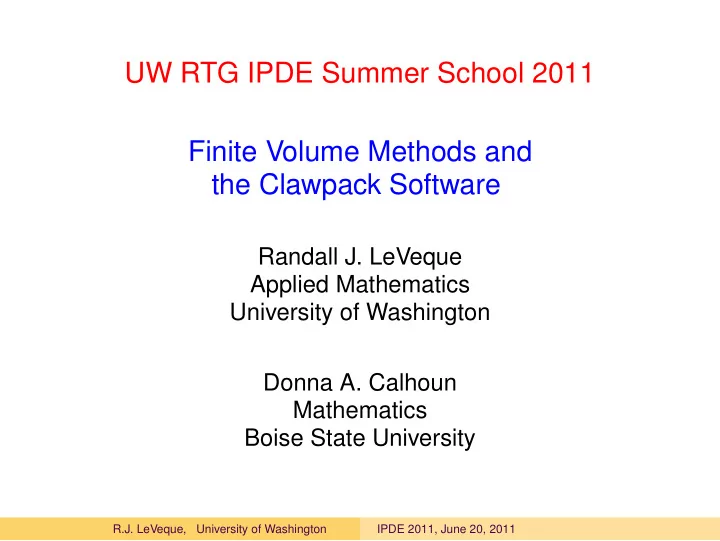
UW RTG IPDE Summer School 2011 Finite Volume Methods and the Clawpack Software Randall J. LeVeque Applied Mathematics University of Washington Donna A. Calhoun Mathematics Boise State University R.J. LeVeque, University of Washington IPDE 2011, June 20, 2011

Course outline Main goals: • Theory of hyperbolic conservation laws in one dimension • Finite volume methods in 1 and 2 dimensions • Some applications: advection, acoustics, Burgers’, shallow water equations, traffic flow • Use of the Clawpack software: www.clawpack.org Slides will be posted and green links can be clicked. $IPDE refers to the webpage http://www.amath.washington.edu/~rjl/ipde R.J. LeVeque, University of Washington IPDE 2011, June 20, 2011

Outline This lecture • Hyperbolic equations • Motivating examples • Advection, flow in a pipe. • Acoustics, sound waves • Elasticity, seismic waves • Shallow water equations, tsunamis Reading: Chapters 1 and 2 Note: Some slides have section numbers on footer. R.J. LeVeque, University of Washington IPDE 2011, June 20, 2011 [FVMHP Chap. 1, 2]

Linear and nonlinear waves A wave is a disturbance or displacement that propagates. Examples: • Water waves (disturbance of depth) • Sound waves (disturbance of pressure) • Seismic waves (displacement of elastic material) R.J. LeVeque, University of Washington IPDE 2011, June 20, 2011

Linear and nonlinear waves A wave is a disturbance or displacement that propagates. Examples: • Water waves (disturbance of depth) • Sound waves (disturbance of pressure) • Seismic waves (displacement of elastic material) Very small disturbances can be modeled by linear partial differential equations Solutions are often continuous, smooth functions R.J. LeVeque, University of Washington IPDE 2011, June 20, 2011

Linear and nonlinear waves A wave is a disturbance or displacement that propagates. Examples: • Water waves (disturbance of depth) • Sound waves (disturbance of pressure) • Seismic waves (displacement of elastic material) Very small disturbances can be modeled by linear partial differential equations Solutions are often continuous, smooth functions Larger displacements require nonlinear equations Solutions may be discontinous: shock waves R.J. LeVeque, University of Washington IPDE 2011, June 20, 2011

First order hyperbolic PDE in 1 space dimension R m , A ∈ l R m × m Linear: q t + Aq x = 0 , q ( x, t ) ∈ l R m (flux) R m → l Conservation law: q t + f ( q ) x = 0 , f : l Quasilinear form: q t + f ′ ( q ) q x = 0 Hyperbolic if A or f ′ ( q ) is diagonalizable with real eigenvalues. Models wave motion or advective transport. Eigenvalues are wave speeds. Note: Second order wave equation p tt = c 2 p xx can be written as a first-order system (acoustics). R.J. LeVeque, University of Washington IPDE 2011, June 20, 2011 [FVMHP Sec. 1.1]

Derivation of Conservation Laws q ( x, t ) = density function for some conserved quantity, so � x 2 q ( x, t ) dx = total mass in interval x 1 changes only because of fluxes at left or right of interval. R.J. LeVeque, University of Washington IPDE 2011, June 20, 2011 [FVMHP Chap. 2]

Derivation of Conservation Laws q ( x, t ) = density function for some conserved quantity. Integral form: � x 2 d q ( x, t ) dx = F 1 ( t ) − F 2 ( t ) dt x 1 where f ( q ) = flux function . F j = f ( q ( x j , t )) , R.J. LeVeque, University of Washington IPDE 2011, June 20, 2011 [FVMHP Chap. 2]

Derivation of Conservation Laws If q is smooth enough, we can rewrite � x 2 d q ( x, t ) dx = f ( q ( x 1 , t )) − f ( q ( x 2 , t )) dt x 1 as � x 2 � x 2 q t dx = − f ( q ) x dx x 1 x 1 or � x 2 ( q t + f ( q ) x ) dx = 0 x 1 True for all x 1 , x 2 = ⇒ differential form: q t + f ( q ) x = 0 . R.J. LeVeque, University of Washington IPDE 2011, June 20, 2011 [FVMHP Chap. 2]

Advection equation Flow in a pipe at constant velocity u = constant flow velocity q ( x, t ) = tracer concentration, f ( q ) = uq = q t + uq x = 0 . ⇒ True solution: q ( x, t ) = q ( x − ut, 0) R.J. LeVeque, University of Washington IPDE 2011, June 20, 2011 [FVMHP Sec. 2.1]

Advection equation Flow in a pipe at constant velocity u = constant flow velocity q ( x, t ) = tracer concentration, f ( q ) = uq = q t + uq x = 0 . ⇒ True solution: q ( x, t ) = q ( x − ut, 0) R.J. LeVeque, University of Washington IPDE 2011, June 20, 2011 [FVMHP Sec. 2.1]

Advection equation Flow in a pipe at constant velocity u = constant flow velocity q ( x, t ) = tracer concentration, f ( q ) = uq = q t + uq x = 0 . ⇒ True solution: q ( x, t ) = q ( x − ut, 0) R.J. LeVeque, University of Washington IPDE 2011, June 20, 2011 [FVMHP Sec. 2.1]

Advection examples Here and on future slides, $IPDE refers to the webpage http://www.amath.washington.edu/~rjl/ipde $CLAW refers to the Clawpack top directory. Examples: • $IPDE/claw-apps/advection-1d-1 Created for this class. • $CLAW/apps/advection Example applications in Clawpack. • $CLAW/book Examples from the book. • www.clawpack.org/doc/apps.html Gallery of applications. R.J. LeVeque, University of Washington IPDE 2011, June 20, 2011

Example: Linear acoustics in a 1d tube � p � p ( x, t ) = pressure perturbation q = u u ( x, t ) = velocity Equations: p t + κu x = 0 κ = bulk modulus ρu t + p x = 0 ρ = density or � p � � p � � � 0 κ + = 0 . u 1 /ρ 0 u t x � Eigenvalues: λ = ± c , where c = κ/ρ = sound speed Second order form: Can combine equations to obtain p tt = c 2 p xx R.J. LeVeque, University of Washington IPDE 2011, June 20, 2011

Riemann Problem Special initial data: � q l if x < 0 q ( x, 0) = q r if x > 0 Example: Acoustics with bursting diaphram Pressure: Acoustic waves propagate with speeds ± c . R.J. LeVeque, University of Washington IPDE 2011, June 20, 2011 [FVMHP Sec. 3.9.1]

Riemann Problem Special initial data: � q l if x < 0 q ( x, 0) = q r if x > 0 Example: Acoustics with bursting diaphram Pressure: Acoustic waves propagate with speeds ± c . R.J. LeVeque, University of Washington IPDE 2011, June 20, 2011 [FVMHP Sec. 3.9.1]

Riemann Problem Special initial data: � q l if x < 0 q ( x, 0) = q r if x > 0 Example: Acoustics with bursting diaphram Pressure: Acoustic waves propagate with speeds ± c . R.J. LeVeque, University of Washington IPDE 2011, June 20, 2011 [FVMHP Sec. 3.9.1]

Riemann Problem Special initial data: � q l if x < 0 q ( x, 0) = q r if x > 0 Example: Acoustics with bursting diaphram Pressure: Acoustic waves propagate with speeds ± c . R.J. LeVeque, University of Washington IPDE 2011, June 20, 2011 [FVMHP Sec. 3.9.1]

Riemann Problem Special initial data: � q l if x < 0 q ( x, 0) = q r if x > 0 Example: Acoustics with bursting diaphram Pressure: Acoustic waves propagate with speeds ± c . R.J. LeVeque, University of Washington IPDE 2011, June 20, 2011 [FVMHP Sec. 3.9.1]

Riemann Problem Special initial data: � q l if x < 0 q ( x, 0) = q r if x > 0 Example: Acoustics with bursting diaphram Pressure: Acoustic waves propagate with speeds ± c . R.J. LeVeque, University of Washington IPDE 2011, June 20, 2011 [FVMHP Sec. 3.9.1]

Riemann Problem for acoustics Waves propagating in x – t space: Left-going wave W 1 = q m − q l and right-going wave W 2 = q r − q m are eigenvectors of A . R.J. LeVeque, University of Washington IPDE 2011, June 20, 2011 [FVMHP Sec. 3.9.1]

Seismic wave in layered medium Red = div(u) [P-waves], Blue = curl(u) [S-waves] R.J. LeVeque, University of Washington IPDE 2011, June 20, 2011

Seismic wave in layered medium Red = div(u) [P-waves], Blue = curl(u) [S-waves] R.J. LeVeque, University of Washington IPDE 2011, June 20, 2011

Seismic wave in layered medium Red = div(u) [P-waves], Blue = curl(u) [S-waves] R.J. LeVeque, University of Washington IPDE 2011, June 20, 2011

Seismic wave in layered medium Red = div(u) [P-waves], Blue = curl(u) [S-waves] R.J. LeVeque, University of Washington IPDE 2011, June 20, 2011

Seismic wave in layered medium Red = div(u) [P-waves], Blue = curl(u) [S-waves] R.J. LeVeque, University of Washington IPDE 2011, June 20, 2011

Seismic wave in layered medium Red = div(u) [P-waves], Blue = curl(u) [S-waves] R.J. LeVeque, University of Washington IPDE 2011, June 20, 2011

Seismic wave in layered medium Red = div(u) [P-waves], Blue = curl(u) [S-waves] R.J. LeVeque, University of Washington IPDE 2011, June 20, 2011

Seismic wave in layered medium Red = div(u) [P-waves], Blue = curl(u) [S-waves] R.J. LeVeque, University of Washington IPDE 2011, June 20, 2011

Seismic wave in layered medium Red = div(u) [P-waves], Blue = curl(u) [S-waves] R.J. LeVeque, University of Washington IPDE 2011, June 20, 2011

Seismic wave in layered medium Red = div(u) [P-waves], Blue = curl(u) [S-waves] R.J. LeVeque, University of Washington IPDE 2011, June 20, 2011

Red = div(u) [P-waves], Blue = curl(u) [S-waves] Four levels with refinement factors 4, 4, 4 R.J. LeVeque, University of Washington IPDE 2011, June 20, 2011

Red = div(u) [P-waves], Blue = curl(u) [S-waves] Four levels with refinement factors 4, 4, 4 R.J. LeVeque, University of Washington IPDE 2011, June 20, 2011