Using BDDs to capture data in Runtime verification (RV) [HP18] Per - - PowerPoint PPT Presentation

Using BDDs to capture data in Runtime verification (RV) [HP18]

Per Ove Ringdal November 29, 2019

Contents

Motivation Syntax and semantics of QTL QTL Example An Efficient Algorithm Using BDDs Summary References

Verifying file operations

Problem: We have a program that writes data to files, and we want to verify that some property always holds. Assume file API which yields the following events:

• pen(f ): file f was open

write(f , d): data d was written to file f close(f ): file f was closed Property: A file should be open when writing data to it.

Runtime Verification - Definition

What is Runtime Verification? ◮ Lightweight formal method that complements classical exhaustive verification techniques [Bar+18] ◮ Analyse a single execution trace of a system ◮ At the price of limited execution coverage, we get precise information on the runtime behavior

Runtime Verification - Analysing execution traces

We analyse the system against a property, yielding an alarm when the property is violated. [HP18] The property for the file API can be written as: ”A file can only be written to if it has been opened in the past, and not closed since then.” Or in Quantified Temporal Logic (QTL), which will be explained later: ∀f ((∃d write(f , d)) → ¬close(f ) S open(f ))

Execution trace examples

Example not valid: {open(f1)} {close(f1)} {write(f1, 2)} valid: {open(f1)} {write(f1, 2)} {close(f1)}

Data reclamation

When data cannot affect the rest of the execution we want to discard this data. For instance, when a file is closed, we can forget that it was

• pened before that

. . . {open(f1)} {close(f1)} Can discard open(f1)

Syntax and semantics of QTL

Syntax and semantics of QTL - Assignment

Definition

Let X be a finite set of variables. An assignment over a set of variables W ⊆ X maps each variable x ∈ W to a value from its associated domain domain(x).

Syntax and semantics of QTL - Assignment

Definition

Let X be a finite set of variables. An assignment over a set of variables W ⊆ X maps each variable x ∈ W to a value from its associated domain domain(x).

Example

[x → 5, y → ”abc”] maps x to 5 and y to ‘abc’.

Syntax and semantics of QTL - Predicate names

Definition

Let T be a set of predicate names, where each predicate name p is associated with some domain domain(p). A predicate is constructed from a predicate name and a variable or a constant of the same type. Predicates over constants are called ground predicates.

Syntax and semantics of QTL - Predicate names

Definition

Let T be a set of predicate names, where each predicate name p is associated with some domain domain(p). A predicate is constructed from a predicate name and a variable or a constant of the same type. Predicates over constants are called ground predicates.

Example

If the predicate name p and the variable x are associated with the domain of strings, we have predicates like p(”gaga”) and p(x),

Syntax and semantics of QTL - Events

Definition

An event is a finite set of ground predicates.

Syntax and semantics of QTL - Events

Definition

An event is a finite set of ground predicates.

Example

If T = {p, q, r}, then {p(”xyzzy”), q(3)} is a possible event.

Syntax and semantics of QTL - Events

Definition

An event is a finite set of ground predicates.

Example

If T = {p, q, r}, then {p(”xyzzy”), q(3)} is a possible event.

Definition

An execution trace σ = s1, s2, . . . is a finite sequence of events.

Syntax and semantics of QTL - Formulas

Definition

The formulas of QTL are defined by the following grammar. ϕ ::= true | p(a) | p(x) | ϕ ∧ ϕ | ¬ϕ | ϕ S ϕ | ⊖ ϕ | ∃x ϕ

Syntax and semantics of QTL - Formulas

Definition

The formulas of QTL are defined by the following grammar. ϕ ::= true | p(a) holds when a is a constant in domain(p) and p(a) occurs in the most recent event | p(x) | ϕ ∧ ϕ | ¬ϕ | ϕ S ϕ | ⊖ ϕ | ∃x ϕ

Syntax and semantics of QTL - Formulas

Definition

The formulas of QTL are defined by the following grammar. ϕ ::= true | p(a) holds when a is a constant in domain(p) and p(a) occurs in the most recent event | p(x) holds with a binding of x to value a if p(a)

• ccurs in the most recent event

| ϕ ∧ ϕ | ¬ϕ | ϕ S ϕ | ⊖ ϕ | ∃x ϕ

Syntax and semantics of QTL - Formulas

Definition

The formulas of QTL are defined by the following grammar. ϕ ::= true | p(a) holds when a is a constant in domain(p) and p(a) occurs in the most recent event | p(x) holds with a binding of x to value a if p(a)

• ccurs in the most recent event

| ϕ ∧ ϕ | ¬ϕ | ϕ S ϕ for ϕ S ψ, ψ held in past or now, and since then ϕ has been true | ⊖ ϕ | ∃x ϕ

Syntax and semantics of QTL - Formulas

Definition

The formulas of QTL are defined by the following grammar. ϕ ::= true | p(a) holds when a is a constant in domain(p) and p(a) occurs in the most recent event | p(x) holds with a binding of x to value a if p(a)

• ccurs in the most recent event

| ϕ ∧ ϕ | ¬ϕ | ϕ S ϕ for ϕ S ψ, ψ held in past or now, and since then ϕ has been true | ⊖ ϕ ϕ is true in the previous event | ∃x ϕ

Syntax and semantics of QTL - Formulas derived

The following formulas can be derived from the definition: false = ¬true ϕ ∨ ψ = ¬(¬ϕ ∧ ¬ψ) ϕ → ψ = ¬ϕ ∧ ψ P ϕ = true S ϕ H ϕ = ¬P ¬ϕ ∀x ϕ = ¬∃x ¬ϕ

Syntax and semantics of QTL - Formulas derived

The following formulas can be derived from the definition: false = ¬true ϕ ∨ ψ = ¬(¬ϕ ∧ ¬ψ) ϕ → ψ = ¬ϕ ∧ ψ P ϕ = true S ϕ ϕ held in the past or now H ϕ = ¬P ¬ϕ ∀x ϕ = ¬∃x ¬ϕ

Syntax and semantics of QTL - Formulas derived

The following formulas can be derived from the definition: false = ¬true ϕ ∨ ψ = ¬(¬ϕ ∧ ¬ψ) ϕ → ψ = ¬ϕ ∧ ψ P ϕ = true S ϕ ϕ held in the past or now H ϕ = ¬P ¬ϕ ϕ always true in the past and now ∀x ϕ = ¬∃x ¬ϕ

Syntax and semantics of QTL - free, hide

Definition

Let free(ϕ) be the set of free (i.e., unquantified) variables of a subformula ϕ.

Syntax and semantics of QTL - free, hide

Definition

Let free(ϕ) be the set of free (i.e., unquantified) variables of a subformula ϕ.

Definition

Let A1 and A2 be sets of assignments. The intersection A1 ∩ A2 is defined like a database ‘join’ operator. The union A1 ∪ A2 is defined as the operator dual of intersection.

Syntax and semantics of QTL - free, hide

Definition

Let free(ϕ) be the set of free (i.e., unquantified) variables of a subformula ϕ.

Definition

Let A1 and A2 be sets of assignments. The intersection A1 ∩ A2 is defined like a database ‘join’ operator. The union A1 ∪ A2 is defined as the operator dual of intersection.

Definition

Let Γ be a set of assignments over a set of variables W. We denote by hide(Γ, x) the sets of assigments over W \ {x}, obtained from Γ by removing the assignment to x for each element of Γ.

Syntax and semantics of QTL - I[ϕ, σ, i]

Definition

Afree(ϕ) is the set of all possible assignments of values to the variables that appear free in ϕ.

Syntax and semantics of QTL - I[ϕ, σ, i]

Definition

Afree(ϕ) is the set of all possible assignments of values to the variables that appear free in ϕ.

Definition

Let I[ϕ, σ, i] be the semantic function, defined below. It returns the set of assignments that satisfy ϕ after the ith event of the exection σ. The empty set of assignments ∅ behaves as the Boolean constant 0 and the singleton set that contains an assignment over an empty set of variables {ǫ} behaves as the Boolean constant 1.

Syntax and semantics of QTL - I[ϕ, σ, i] cont.

I[ϕ, σ, 0] = ∅ I[true, σ, i] = {ǫ} I[p(a), σ, i] = if p(a) ∈ σ[i] then {ǫ} else ∅ I[p(x), σ, i] = {[x → a] | p(a) ∈ σ[i]} I[ϕ ∧ ψ, σ, i] = I[ϕ, σ, i] ∩ I[ψ, σ, i] I[¬ϕ, σ, i] = Afree(ϕ) \ I[ϕ, σ, i] I[ϕ S ψ, σ, i] = I[ψ, σ, i] ∪ (I[ϕ, σ, i] ∩ I[ϕ S ψ, σ, i − 1]) I[⊖ ϕ, σ, i] = I[ϕ, σ, i − 1] I[∃x ϕ, σ, i] = hide(I[ϕ, σ, i], x)

QTL Example

An Efficient Algorithm Using BDDs

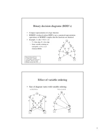
Boolean functions as Binary Decision Diagrams

Here Ordered Binary Decision Diagrams (OBDD) are used. BDDs are a way of efficiently representing a boolean function (f : 2n → 2) as a directed asyclic graph.

1 BDD(⊤): a 1 a: a b 1 a ∧ b:

Algorithm for monitoring QTL

• 1. Initially, for each subformula ϕ, now(ϕ) := BDD(⊥)
• 2. Observe a new event (as set of ground predicates) s as input
• 3. Let pre := now
• 4. Make the following updates for each subformula. If ϕ is a

subformula of ψ then now(ϕ) is updated before now(ψ)

◮ now(true) := BDD(⊤) ◮ now(p(a)) := if p(a) ∈ s then BDD(⊤) else BDD(⊥) ◮ now(p(x)) := build(x, V ) where V = {a | p(a) ∈ s} ◮ now(ϕ ∧ ψ) := and(now(ϕ), now(ψ)) ◮ now(¬ϕ) := not(now(ϕ)) ◮ now(ϕ S ψ) := or(now(ψ), and(now(ϕ), pre(ϕ S ψ))) ◮ now(⊖ ϕ) := pre(ϕ) ◮ now(∃x ϕ) := exists(x0, . . . , xk−1, now(ϕ))

• 5. Goto step 2

Summary

◮ First-order past time temporal logic properties (QTL) ◮ The properties contains data (ground predicates) over infinite domains

References I

Ezio Bartocci et al. “Introduction to Runtime Verification”. In: Lectures on Runtime Verification: Introductory and Advanced Topics. Ed. by Ezio Bartocci and Yli` es Falcone. Cham: Springer International Publishing, 2018, pp. 1–33. isbn: 978-3-319-75632-5. doi: 10.1007/978-3-319-75632-5_1. url: https://doi.org/10.1007/978-3-319-75632-5_1. Klaus Havelund and Doron Peled. “BDDs on the Run”. In: Leveraging Applications of Formal Methods, Verification and Validation. Industrial Practice. Ed. by Tiziana Margaria and Bernhard Steffen. Cham: Springer International Publishing, 2018, pp. 58–69. isbn: 978-3-030-03427-6. url: https: //link.springer.com/chapter/10.1007%2F978-3- 030-03427-6_8.