Unsupervised learning General introduction to unsupervised learning - PowerPoint PPT Presentation
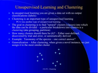
Unsupervised learning General introduction to unsupervised learning PCA Special directions These are special directions we will try to find. Best direction u : |u| 2 = 1 2 1. Minimize : d i X i T u is the projection length x i u d i T
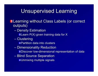
Unsupervised learning • General introduction to unsupervised learning
PCA
Special directions These are special directions we will try to find.
Best direction u : |u| 2 = 1 2 1. Minimize : Σd i X i T u is the projection length x i u d i T u) 2 2. Maximize : Σ ( x i u is the direction that maximizes the variance
Finding the best projection: X i u d i Find u that maximize : Σ ( x i T u) 2 T 2 T T ( x u ) = ( u x ) ( x u ) i max Σ ( u T x i ) (x i T u) T = max u [V] u where: [V] = Σ (x i x i T )
The data matrix: X X T [V] = [V ] = Σ (x i x i T ) = XX T
Best direction u • Will minimize the distances from it • Will maximize the variance along it Max(u): u T [V] u subject to: |u| = 1 With Lagrange multipliers: d/dx (x T U x) = 2Ux Maximize u T [V] u - λ( u T u – 1) d/dx (x T x) = 2x Derivative with respect to the vector u: [V]u – λ u = 0 [V]u = λ u The best direction will be the first eigenvector of [V]
Best direction u: X i u d i The best direction will be the first eigenvector of [V]; u 1 with variance λ 1 The next direction will be the second eigenvector of [V]; u 2 with variance λ 2 The Principle Components will be the eigenvectors of the data matrix
PCs, Variance and Least-Squares • The first PC retains the greatest amount of variation in the sample • The k th PC retains the k th greatest fraction of the variation in the sample • The k th largest eigenvalue of the correlation matrix C is the variance in the sample along the k th PC • The least-squares view: PCs are a series of linear least squares fits to a sample, each orthogonal to all previous ones
Dimensionality Reduction Can ignore the components of lesser significance. 25 20 Scree plot Variance (%) 15 10 5 0 PC1 PC2 PC3 PC4 PC5 PC6 PC7 PC8 PC9 PC10 You do lose some information, but if the eigenvalues are small, you don’t lose much – n dimensions in original data – calculate n eigenvectors and eigenvalues – choose only the first k eigenvectors, based on their eigenvalues – final data set has only k dimensions
PC dimensionality reduction In the linear case only
PCA and correlations • We can think of our data points as k points from a distribution p(x) • We have k samples (x 1 y 1 ) (x 2 y 2 )… …( x k y k )
PCA and correlations • We have k samples (x 1 y 1 ) (x 2 y 2 )… …( x k y k ) • The correlation between(x,y) is: E [ (x-x 0 ) (y – y 0 ) / σ x σ y ] • For centered variables, x,y are uncorrelated if E(xy) = 0
v 2 v 1 Correlation depends on the coordinates: (x,y) are correlated, (v 1 v 2 ) are not
In the PC coordinates, the variables are uncorrelated • T v 1 T x i ). The projection of a point x i on v 1 is: x i (or v 1 • T v 2 The projection of a point x i on v 2 is: x i • For the correlation, we take the sum: Σ i ( v 1 T v 2 ) T x i ) (x i • Σ i v 1 T x i x i T v 2 = v 1 T C v 2 = • Where C = X T X. (the data matrix) • C v 2 = λ 2 v 2 Since the v i are eigenvectors of C, • • T C v 2 = λ 2 v 1 T v 2 = 0 v 1 • The variables are uncorrelated. • This is a result of using as coordinates the eigenvectors of the correlation matrix C = X T X.
In the PC coordinates the variables are uncorrelated • The correlation depends on the coordinate system. We can start with variables (x,y) which are correlated, transform them to (x', y') that will be un-correlated • If we use the coordinates defined by the eigenvectors of XX T the variables (or the vectors x i of n projections on the i'th axis) will be uncorrelated.
Properties of the PCA • The subspace spanned by the first k PC retains the maximal variance • This subspace minimized the distance of the points from the subspace • The transformed variables, which are linear combinations of the original ones, are uncorrelated.
Best plane, minimizing perpendicular distance over all planes
Eigenfaces: PC of face images • Turk, M., Pentland, A.: Eigenfaces for recognition . J. Cognitive Neuroscience 3 (1991) 71 – 86.
Image Representation • Training set of m images of size N*N are represented by vectors of size N 2 x 1 ,x 2 ,x 3 ,…, x M Example 1 2 3 1 2 3 3 3 1 2 1 4 5 1 3 3 2 4 Need to be well aligned 5 1 9 1
Average Image and Difference Images • The average training set is defined by m = (1 /m) ∑ m i=1 x i • Each face differs from the average by vector r i = x i – m
Covariance Matrix • The covariance matrix is constructed as T where A=[r 1 ,…, r m ] C = AA Size of this matrix is N 2 x N 2 • Finding eigenvectors of N 2 x N 2 matrix is intractable. Hence, use the matrix A T A of size m x m and find eigenvectors of this small matrix.
Face data matrix: m X T m N 2 N 2 X XX T is N 2 * N 2 X T X is m * m
Eigenvectors of Covariance Matrix • Consider the eigenvectors v i of A T A such that A T A v i = m i v i • Pre-multiplying both sides by A , we have AA T ( A v i ) = m i ( A v i ) • A v i is an eigenvector of our original AA T • Find the eigenvectors v i of the small A T A • Get the ‘ eigen- faces’ by A v i
Face Space • u i resemble facial images which look ghostly, hence called Eigenfaces
Projection into Face Space • A face image can be projected into this face space by p k = U T (x k – m ) Rows of U T are the eigenfaces p k are the m coefficients of face x k This is the representation of a face using eigen-faces This representation can then be used for recognition using different recognition algorithms
Recognition in ‘face space’ • Turk and Pentland used 16 faces, and 7 pc • In this case the face representation p: p k = U T (x k – m ) is 7-long vector • • Face classification: • Several images per face-class. • For a new test image I: obtain the representation p I • Turk-Pentland used simple nearest neighbor • Find NN in each class, take the nearest, • s.t. distance < ε, otherwise result is ‘unknown’ • Other algorithms are possible, e.g. SVM
Face detection by ‘face space’ • Turk-Pentland used ‘ faceness ’ measure: • Within a window, compare the original image with its reconstruction from face-space • Find the distance Є between the original image x and its reconstructed image from the eigenface space, x f , Є 2 = || x – x f || 2 , where x f = Up + μ (reconstructed face) • If ε < θ for a threshold θ • A face is detected in the window • Not ‘state -of-the-art and not fast enough • Eigenfaces in the brain?
Next: PCA by Neurons
Recommend
More recommend
Explore More Topics
Stay informed with curated content and fresh updates.
