Tutorial 2 the outline Example-1 from linear algebra Conditional - PowerPoint PPT Presentation
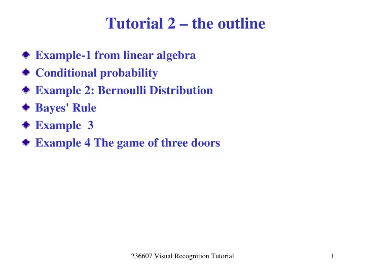
Tutorial 2 the outline Example-1 from linear algebra Conditional probability Example 2: Bernoulli Distribution Bayes' Rule Example 3 Example 4 The game of three doors 236607 Visual Recognition Tutorial 1 Example 1: Linear Algebra A
Tutorial 2 – the outline Example-1 from linear algebra Conditional probability Example 2: Bernoulli Distribution Bayes' Rule Example 3 Example 4 The game of three doors 236607 Visual Recognition Tutorial 1
Example – 1: Linear Algebra A line can be written as ax+by=1 . You are given a number of example points: ⎡ ⎤ x y 1 1 ⎢ ⎥ = M M P ⎢ ⎥ ⎢ ⎥ ⎣ x y ⎦ ⎡ ⎤ a n n = ⎢ ⎥ Let M ⎣ ⎦ b • (A) Write a single matrix equation that expresses the constraint that each of these points lies on a single line • (B) Is it always the case that some M exists? • (C) Write an expression for M assuming it does exist. 236607 Visual Recognition Tutorial 2
Example – 1: Linear Algebra (A) For all the points to lie on the line, a and b must satisfy the following set of simultaneous equations: ax 1 +by 1 =1 : ax N +by N =1 This can be written much more compactly in the matrix form (linear regression equation): PM = 1 where 1 is an Nx1 column vector of 1’s. (B) An M satisfying the matrix equation in part (A) will not exist unless al the points are collinear (i.e. fall on the same line). In general, three or more points may not be collinear. (C) If M exists, then we can find it by finding the left inverse of P , but since P is in general not a square matrix P -1 may not exist, so we need the pseudo-inverse ( P T P ) -1 P T . Thus M= ( P T P ) -1 P T 1. 236607 Visual Recognition Tutorial 3
Conditional probability When 2 variables are statistically dependent, knowing the value of one of them lets us get a better estimate of the value of the other one. This is expressed by the conditional probability of x given y : = = Pr{ x v y , w } P x y ( , ) = = = = i j Pr{ x v | y w } , or ( | ) P x y = i j Pr{ y w } P y ( ) j y = If x and y are statistically independent, then P x y ( | ) P x ( ). x 236607 Visual Recognition Tutorial 4
Bayes' Rule • The law of total probability : If event A can occur in m different ways A 1 ,A 2 ,…,A m and if they are mutually exclusive,then the probability of A occurring is the sum of the probabilities A 1 ,A 2 ,…,A m . = ∑ P y ( ) P x y ( , ). ∈ χ x From definition of condition probability = = Px y ( , ) Px y P y ( | ) ( ) P y x Px ( | ) ( ) 236607 Visual Recognition Tutorial 5
Bayes' Rule P y x P x ( | ) ( ) = x P x y ( | ) P y ( ) or P y x P x ( | ) ( ) P y x P x ( | ) ( ) = = P x y ( | ) ∑ ∑ P x y ( , ) P y x P x ( | ) ( ) ∈ χ ∈ χ x x × likelihood prior = posterior evidence 236607 Visual Recognition Tutorial 6
Bayes' rule – continuous case • For continuous random variable we refer to densities rather than probabilities; in particular, p x y ( , ) = p x y ( | ) p y ( ) • The Bayes’ rule for densities becomes: p y x p x ( | ) ( ) = p x y ( | ) ∞ ∫ p y x p x dx ( | ) ( ) −∞ 236607 Visual Recognition Tutorial 7
Bayes' formula - importance � Call x a ‘cause’, y an effect. Assuming x is present, we know the likelihood of y to be observed � The Bayes’ rule allows to determine the likelihood of a cause x given an observation y. (Note that there may be many causes producing y ). � The Bayes’ rule shows how probability for x changes from prior p( x ) before we observe anything, to posterior p(x| y) once we have observed y. 236607 Visual Recognition Tutorial 8
Example – 2: Bernoulli Distribution A random variable X has a Bernoulli distribution with parameter θ if it can assume a value of 1 with a probability of θ and the value of 0 with a probability of (1- θ ). The random variable X is also known as a Bernoulli variable with parameter θ and has the following probability mass function: θ =1 ⎧ x θ = ⎨ − = 0 ( , ) x p θ ⎩ 1 x The mean of a random variable X that has a Bernoulli distribution with parameter p is E(X) = 1( θ ) + 0(1- θ ) = θ The variance of X is 236607 Visual Recognition Tutorial 9
Example – 2: Bernoulli Distribution = − = θ + − θ − θ = θ − θ = θ − θ 2 2 2 2 2 2 Var X ( ) E X ( ) [ ( E X )] 1 ( ) 0 (1 ) (1 ) A random variable whose value represents the outcome of a coin toss (1 for heads, 0 for tails, or vice-versa) is a Bernoulli variable with parameter θ , where θ is the probability that the outcome corresponding to the value 1 occurs. For an unbiased coin, where heads or tails are equally likely to occur, θ = 0.5. For Bernoulli rand. variable x n the probability mass function is: − θ = = θ − θ = 0,1 x 1 x P x ( | ) P x ( ) (1 ) , x n n θ n n n For N independent Bernoulli trials we have random sample = ( x x , ,..., x ) x − 0 1 N 1 236607 Visual Recognition Tutorial 10
Example – 2: Bernoulli Distribution The distribution of the random sample is: − N 1 ∏ − = θ − θ = θ − θ − x 1 x k N k P ( ) (1 ) (1 ) x n n θ = n 0 − N 1 ∑ = ∈ = k x number of ones x ( x x , ,..., x ). − n 0 1 N 1 = n 0 The distribution of the number of ones in N independent Bernoulli trials is: ⎛ ⎞ N = θ − θ − k N k P k ( ) ⎜ ⎟ (1 ) θ ⎝ ⎠ k The joint probability to observe the sample x and the number k = ∈ ⎧ P ( ), k number of ones x x θ = ⎨ P ( , ) k x θ ⎩ 0, otherwise 236607 Visual Recognition Tutorial 11
Example – 2: Bernoulli Distribution The conditional probability of x given the number k of ones: − θ − θ k N k P ( , ) k (1 ) 1 x = = = θ P ( | ) k x θ ⎛ ⎞ ⎛ ⎞ N N P k ( ) − θ θ − θ k N k (1 ) ⎜ ⎟ ⎜ ⎟ ⎝ k ⎠ ⎝ k ⎠ Thus 1 = = ⎛ P ( ) P ( | ) k P k ( ) P k ( ) x x θ θ θ θ ⎞ N ⎜ ⎟ ⎝ k ⎠ 236607 Visual Recognition Tutorial 12
Example - 3 Assume that X is distributed according to the Gaussian density with mean μ =0 and variance σ 2 =1 . • (A) What is the probability that x =0 ? Assume that Y is distributed according to the Gaussian density with mean μ =1 and variance σ 2 =1 . • (B) What is the probability that y =0 ? Given a distribution: Pr(Z=z)=1/2Pr(X=z)+1/2Pr(Y=z) known as a mixture (i.e. ½ of the time points are generated by the X process and ½ of the time points by the Y process ). • (C) If Z =0, what is the probability that the X process generated this data point ? 236607 Visual Recognition Tutorial 13
Example – 3 solutions (A) Since p(x) is a continuous density, the probability that x=0 0 is ∫ < ≤ = = Pr(0 x 0) p x dx ( ) 0. 0 (B) As in part (A) , the probability that y=0 is 0 ∫ < ≤ = = Pr(0 y 0) p y dy ( ) 0. 0 (C) Let ω 0 ( ω 1 ) be the state where the X ( Y ) process generates a data point. We want Pr( ω 0 |Z=0 ). Using Bayes’ rule and working with the probability densities to get the total probability: 236607 Visual Recognition Tutorial 14
Example - 3 = ω ω = ω ω p Z ( 0 | )Pr( ) p Z ( 0 | )Pr( ) ω = = = 0 0 0 0 Pr( | Z 0) = = ω ω + = ω ω 0 p Z ( 0) p Z ( 0 | )Pr( ) p Z ( 0 | )Pr( ) 0 0 1 1 = = 0.5 p ( X 0) p ( X 0) = = X X = + = = + = 0.5 p ( X 0) 0.5 p Y ( 0) p ( X 0) p Y ( 0) X Y X Y 0.3989 = = 0.6224 + 0.3989 0.2420 where 1 1 2 2 − − − ( y 1) x = , = p ( ) x e p ( ) y e 2 2 X Y π π 2 2 236607 Visual Recognition Tutorial 15
Example 4 The game of three doors A game: 3 doors, there is a prize behind one of them. You have to select one door. Then one of the other two doors is opened (not revealing the prize). At this point you may either stick with your door, or switch to the other (still closed) door. Should one stick with his initial choice, or switch, and does your choice make any difference at all? 236607 Visual Recognition Tutorial 16
The game of three doors Let H i denote the hypothesis “the prize is behind the door i ”. 1 = = = Assumption: Pr( H ) Pr( H ) Pr( H ) 1 2 3 3 Suppose w.l.o.g.: initial choice of door 1,then door 3 is opened. We can stick with 1 or switch to 2. Let D denote the door which is opened by the host. We 1 = = = = = = assume: Pr( D 2 | H ) ,Pr( D 2 | H ) 0,Pr( D 2 | H ) 1, 1 2 3 2 1 = = = = = = Pr( D 3| H ) ,Pr( D 3| H ) 1,Pr( D 3| H ) 0 1 2 3 2 By Bayes’ formula: = Pr( D 3| H )Pr( H ) = = i i Pr( H | D 3) , i = Pr( D 3) 1 1 1 1 2 3 3 = = = = = = Pr( H | D 3) ,Pr( H | D 3) ,Pr( H | D 3) 0 1 = 2 = 3 Pr( D 3) Pr( D 3) 236607 Visual Recognition Tutorial 17
The game of three doors-the solutiion 1 The denominator is a normalizing factor. D = = Pr( 3) 2 So we get 1 = = Pr( H | D 3) , 1 2 2 = = Pr( H | D 3) , 2 3 = = Pr( H | D 3) 0, 3 which means that we are more likely to win the prize if we switch to the door 2. 236607 Visual Recognition Tutorial 18
Recommend
More recommend
Explore More Topics
Stay informed with curated content and fresh updates.
