Time Series Regression A regression model relates a response x t to - PowerPoint PPT Presentation

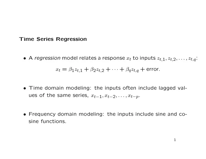
Time Series Regression • A regression model relates a response x t to inputs z t, 1 , z t, 2 , . . . , z t,q : x t = β 1 z t, 1 + β 2 z t, 2 + · · · + β q z t,q + error . • Time domain modeling: the inputs often include lagged val- ues of the same series, x t − 1 , x t − 2 , . . . , x t − p . • Frequency domain modeling: the inputs include sine and co- sine functions. 1

Fitting a Trend > g1900 = window(globtemp, start = 1900) > plot(g1900) window(globtemp, start = 1900) 0.4 0.2 0.0 −0.4 1900 1920 1940 1960 1980 2000 Time 2

• possible model: x t = β 1 + β 2 t + w t , where the error (“noise”) is white noise (unlikely!). • fit using ordinary least squares (OLS): > lmg1900 = lm(g1900 ~ time(g1900)); summary(lmg1900) Call: lm(formula = g1900 ~ time(g1900)) Residuals: Min 1Q Median 3Q Max -0.30352 -0.09671 0.01132 0.08289 0.33519 3

Coefficients: Estimate Std. Error t value Pr(>|t|) (Intercept) -1.219e+01 9.032e-01 -13.49 <2e-16 *** time(g1900) 6.209e-03 4.635e-04 13.40 <2e-16 *** --- Signif. codes: 0 *** 0.001 ** 0.01 * 0.05 . 0.1 1 Residual standard error: 0.1298 on 96 degrees of freedom Multiple R-Squared: 0.6515, Adjusted R-squared: 0.6479 F-statistic: 179.5 on 1 and 96 DF, p-value: < 2.2e-16 4

> plot(g1900) > abline(reg = lmg1900) 0.4 0.2 g1900 0.0 −0.4 1900 1920 1940 1960 1980 2000 Time 5

Using PROC ARIMA Program data globtemp; infile ’globtemp.dat’; n + 1; input globtemp; year = 1855 + n; run; proc arima data = globtemp; where year >= 1900; identify var = globtemp crosscorr = year; /* The ESTIMATE statement fits a model to the *\ \* variable in the most recent IDENTIFY statement */ estimate input = year; run; and output. 6

Regression Review • the regression model: x t = β 1 z t, 1 + β 2 z t, 2 + · · · + β q z t,q + w t = β ′ z t + w t . • fit by minimizing the residual sum of squares n � 2 � � x t − β ′ z t RSS( β ) = t =1 • find the minimum by solving the normal equations   n n  ˆ � z t z ′ � β = z t x t . t  t =1 t =1 7

Matrix Formulation • factor matrix Z n × q = ( z 1 , z 2 , . . . , z n ) ′ , response vector x n × 1 = ( x 1 , x 2 , . . . , x n ) ′ β = ( Z ′ Z ) − 1 Z ′ x • normal equations ( Z ′ Z )ˆ β = Z ′ x with solution ˆ • minimized RSS � ′ � � ˆ � � � x − Z ˆ x − Z ˆ RSS = β β β β ′ Z ′ x = x ′ x − ˆ = x ′ x − x ′ Z ( Z ′ Z ) − 1 Z ′ x 8

Distributions • If the (white noise) errors are normally distributed ( w t ∼ iid N(0 , σ 2 w )), then ˆ β is multivariate normal, and the usual t - and F -statistics have the corresponding distributions. • If the errors are not normally distributed, but still iid, the same is approximately true. • If the errors are not white noise, none of that is true. 9

Choosing a Regression Model • We want a model that fits well without using too many pa- rameters. • Two estimates of the noise variance: – unbiased: s 2 w = RSS / ( n − q ) σ 2 = RSS /n . – maximum likelihood: ˆ σ 2 but also small q . • We want small ˆ 10

Information Criteria (smaller is better) • Akaike’s Information Criterion (with k variables in the model): k + n + 2 k σ 2 AIC = ln ˆ n • bias-corrected Akaike’s Information Criterion: n + k σ 2 AICc = ln ˆ k + n − k − 2 • Schwarz’s (Bayesian) Information Criterion: k + k ln n σ 2 SIC = ln ˆ n 11

Notes • More commonly (e.g. in SAS output and in R’s AIC function), these are all multiplied by n . • AIC, AICc, and SIC (also known as SBC and BIC) can be generalized to other problems where likelihood methods are used. • If n is large and the true k is small, minimizing BIC picks k well, but minimizing AIC tends to over-estimate it. • If the true k is large (or infinite), minimizing AIC picks a value that gives good predictions by trading off bias vs variance. 12