Fitting Regression Models A multiple regression model relates a - PowerPoint PPT Presentation

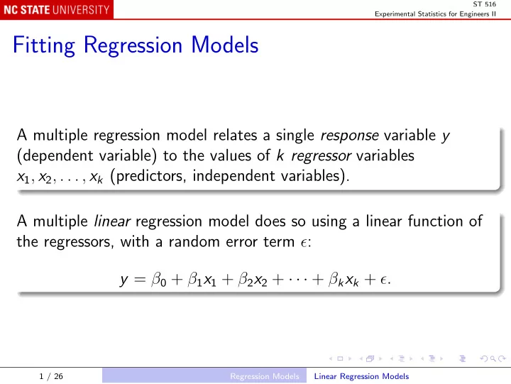
ST 516 Experimental Statistics for Engineers II Fitting Regression Models A multiple regression model relates a single response variable y (dependent variable) to the values of k regressor variables x 1 , x 2 , . . . , x k (predictors, independent variables). A multiple linear regression model does so using a linear function of the regressors, with a random error term ǫ : y = β 0 + β 1 x 1 + β 2 x 2 + · · · + β k x k + ǫ. 1 / 26 Regression Models Linear Regression Models

ST 516 Experimental Statistics for Engineers II The model is called linear because it is a linear function of the unknown parameters β 0 , β 1 , . . . , β k . However, some x ’s may be functions of others. For instance, y = β 0 + β 1 x 1 + β 2 x 2 + β 3 x 1 x 2 + ǫ. and y = β 0 + β 1 x 1 + β 2 x 2 + β 3 x 2 1 + β 4 x 1 x 2 + β 5 x 2 2 + ǫ. are both linear regression models. 2 / 26 Regression Models Linear Regression Models

ST 516 Experimental Statistics for Engineers II Parameter Estimation Inference Suppose we have n observations of the response, y 1 , y 2 , . . . , y n corresponding values of the regressors; x i , j is the value of the j th regressor associated with the i th observation. Assume that E( ǫ ) = 0 and V( ǫ ) = σ 2 . What can we say (infer) about β 0 , β 1 , . . . , β k ? 3 / 26 Regression Models Parameter Estimation

ST 516 Experimental Statistics for Engineers II Method of least squares : the best values of the parameters are the ones that minimize � 2 � n n k � ǫ 2 � � L = i = y i − β 0 − β j x i , j . i =1 i =1 j =1 L is a quadratic function of β 0 , β 1 , . . . , β k , so we can find the minimum by equating the gradient to 0 . We obtain p = k + 1 linear equations (the normal equations) in the p unknowns. 4 / 26 Regression Models Parameter Estimation

ST 516 Experimental Statistics for Engineers II The equations may be written compactly in terms of vectors and matrices:       y 1 1 x 1 , 1 x 1 , 2 . . . x 1 , k β 0 1 y 2 x 2 , 1 x 2 , 2 . . . x 2 , k β 1       y =  , X =  , β =  , . . . . . .       . . . . . .  .   . . . .   .     y n 1 x n , 1 x n , 2 . . . x n , k β k and   ǫ 1 ǫ 2   ǫ =  . .   .  .   ǫ n 5 / 26 Regression Models Parameter Estimation

ST 516 Experimental Statistics for Engineers II In terms of these vectors and matrices, the model may be written y = X β + ǫ , and the normal equations are X ′ X ˆ β = X ′ y . 6 / 26 Regression Models Parameter Estimation

ST 516 Experimental Statistics for Engineers II If X ′ X is non-singular, and hence has an inverse, the normal equations may be solved to give β = ( X ′ X ) − 1 X ′ y . ˆ If not, the equations still have solutions, but they are not unique. The fitted values and residuals are y = X ˆ ˆ and e = y − ˆ y , β and are unique even when ˆ β is not. 7 / 26 Regression Models Parameter Estimation

ST 516 Experimental Statistics for Engineers II Estimating σ 2 The residual sum of squares is n n y i ) 2 = � � i = e ′ e = y ′ y − ˆ ′ X ′ y . e 2 SS E = ( y i − ˆ β i =1 i =1 We can show that SS E has n − p degrees of freedom, and E(SS E ) = ( n − p ) σ 2 , so that the corresponding mean square σ 2 = SS E ˆ n − p is an unbiased estimator of σ 2 . 8 / 26 Regression Models Parameter Estimation

ST 516 Experimental Statistics for Engineers II Properties of ˆ β Unbiasedness: � � ˆ E β = β . Variances and covariances: � � � � � �  ˆ β 0 , ˆ ˆ β 0 , ˆ ˆ  V β 0 Cov β 1 . . . Cov β k � � � � � �  β 1 , ˆ ˆ ˆ β 1 , ˆ ˆ  Cov V Cov β 0 β 1 . . . β k � �   ˆ Cov β =   . . . ...  . . .  . . .     � � � � � � β k , ˆ ˆ β k , ˆ ˆ ˆ Cov β 0 Cov β 1 . . . V β k = σ 2 ( X ′ X ) − 1 . 9 / 26 Regression Models Parameter Estimation

ST 516 Experimental Statistics for Engineers II Example: Viscosity of a polymer viscosity.txt Temperature CatalystFeedRate Viscosity 80 8 2256 93 9 2340 100 10 2426 82 12 2293 90 11 2330 99 8 2368 81 8 2250 96 10 2409 94 12 2364 93 11 2379 97 13 2440 95 11 2364 100 8 2404 85 12 2317 86 9 2309 87 12 2328 10 / 26 Regression Models Parameter Estimation

ST 516 Experimental Statistics for Engineers II R commands viscosity <- read.table("data/viscosity.txt", header = TRUE) viscosityLm <- lm(Viscosity ~ Temperature + CatalystFeedRate, viscosity) summary(viscosityLm) Output Call: lm(formula = Viscosity ~ Temperature + CatalystFeedRate, data = viscosity) Residuals: Min 1Q Median 3Q Max -21.4972 -13.1978 -0.4736 10.5558 25.4299 11 / 26 Regression Models Parameter Estimation

ST 516 Experimental Statistics for Engineers II Output, continued Coefficients: Estimate Std. Error t value Pr(>|t|) (Intercept) 1566.0778 61.5918 25.43 1.80e-12 *** Temperature 7.6213 0.6184 12.32 1.52e-08 *** CatalystFeedRate 8.5848 2.4387 3.52 0.00376 ** --- Signif. codes: 0 *** 0.001 ** 0.01 * 0.05 . 0.1 1 Residual standard error: 16.36 on 13 degrees of freedom Multiple R-Squared: 0.927, Adjusted R-squared: 0.9157 F-statistic: 82.5 on 2 and 13 DF, p-value: 4.1e-08 Fitted model is y = 1566 . 0778 ˆ + 7 . 6213 (0 . 6184) x 1 + 8 . 5848 (2 . 4387) x 2 . (61 . 5918) 12 / 26 Regression Models Parameter Estimation

ST 516 Experimental Statistics for Engineers II Residual plots Make four plots of the residuals: plot(viscosityLm) The first three are the usual (Residuals vs. fitted, Q-Q, and Scale-Location), but the fourth now displays residuals vs. leverage . 13 / 26 Regression Models Parameter Estimation

ST 516 Experimental Statistics for Engineers II Residuals vs Fitted 30 8 ● 11 ● 20 ● ● 10 ● ● ● Residuals 0 ● ● ● ● −10 ● ● −20 ● ● ● 9 2250 2300 2350 2400 Fitted values lm(Viscosity ~ Temperature + CatalystFeedRate) 14 / 26 Regression Models Parameter Estimation

ST 516 Experimental Statistics for Engineers II Normal Q−Q 2.0 11 8 ● ● 1.5 1.0 ● ● Standardized residuals ● ● 0.5 ● 0.0 ● ● ● ● −0.5 ● −1.0 ● ● −1.5 ● 6 ● −2 −1 0 1 2 Theoretical Quantiles lm(Viscosity ~ Temperature + CatalystFeedRate) 15 / 26 Regression Models Parameter Estimation

ST 516 Experimental Statistics for Engineers II Scale−Location 11 ● ● 8 6 ● 1.2 ● ● 1.0 ● ● ● ● Standardized residuals 0.8 ● ● ● 0.6 ● 0.4 ● ● 0.2 ● 0.0 2250 2300 2350 2400 Fitted values lm(Viscosity ~ Temperature + CatalystFeedRate) 16 / 26 Regression Models Parameter Estimation

ST 516 Experimental Statistics for Engineers II Residuals vs Leverage 2 11 ● ● 0.5 1 1 ● ● Standardized residuals ● ● ● 0 ● ● ● ● ● −1 ● ● ● ● 6 0.5 Cook's distance 0.00 0.05 0.10 0.15 0.20 0.25 0.30 0.35 Leverage lm(Viscosity ~ Temperature + CatalystFeedRate) 17 / 26 Regression Models Parameter Estimation

ST 516 Experimental Statistics for Engineers II Regression and Factorial Designs We have used regression to find main effects and interactions in experiments with factorial (full and partial) designs, as an alternative to the hand calculation of effects and the ANOVA table. If some observations are missing in a factorial design, unbiased estimates of effects can be calculated only using regression methods. 18 / 26 Regression Models Parameter Estimation

ST 516 Experimental Statistics for Engineers II Example A 2 3 design with 4 center points (yield-10-2.txt): Temperature Pressure Catalyst Yield -1 -1 -1 32 1 -1 -1 46 -1 1 -1 57 1 1 -1 65 -1 -1 1 36 1 -1 1 48 -1 1 1 57 1 1 1 68 0 0 0 50 0 0 0 44 0 0 0 53 0 0 0 56 19 / 26 Regression Models Parameter Estimation

ST 516 Experimental Statistics for Engineers II R commands ex10p2 <- read.table("data/yield-10-2.txt", header = TRUE) summary(lm(Yield ~ Temperature + Pressure + Catalyst, ex10p2)) Output Call: lm(formula = Yield ~ Temperature + Pressure + Catalyst, data = ex10p2) Residuals: Min 1Q Median 3Q Max -7.000e+00 -1.031e+00 -3.483e-15 1.344e+00 5.000e+00 Coefficients: Estimate Std. Error t value Pr(>|t|) (Intercept) 51.0000 0.9662 52.783 1.84e-11 *** Temperature 5.6250 1.1834 4.753 0.00144 ** Pressure 10.6250 1.1834 8.979 1.89e-05 *** Catalyst 1.1250 1.1834 0.951 0.36961 --- Signif. codes: 0 *** 0.001 ** 0.01 * 0.05 . 0.1 1 Residual standard error: 3.347 on 8 degrees of freedom Multiple R-squared: 0.9286, Adjusted R-squared: 0.9019 F-statistic: 34.7 on 3 and 8 DF, p-value: 6.196e-05 20 / 26 Regression Models Parameter Estimation