Thus far we have emphasized: 1. Writing the likelihood equation. L ( - PDF document

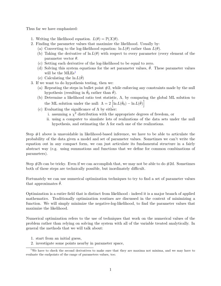
Thus far we have emphasized: 1. Writing the likelihood equation. L ( θ ) = P ( X | θ ). 2. Finding the parameter values that maximize the likelihood. Usually by: (a) Converting to the log-likelihood equation: ln L ( θ ) rather than L ( θ ). (b) Taking the derivative of ln L ( θ ) with respect to every parameter (every element of the parameter vector θ . (c) Setting each derivative of the log-likelihood to be equal to zero. (d) Solving this system equations for the set parameter values, ˆ θ . These parameter values will be the MLEs 1 (e) Calculating the ln L (ˆ θ ) 3. If we want to do hypothesis testing, then we: (a) Repeating the steps in bullet point #2, while enforcing any constraints made by the null hypothesis (resulting in ˆ θ 0 rather than ˆ θ ). (b) Determine a likelihood ratio test statistic, Λ, by comparing the global ML solution to � � ln L (ˆ θ 0 ) − ln L (ˆ the ML solution under the null: Λ = 2 θ ) (c) Evaluating the significance of Λ by either: i. assuming a χ 2 distribution with the appropriate degrees of freedom, or ii. using a computer to simulate lots of realizations of the data sets under the null hypothesis, and estimating the Λ for each one of the realizations. Step #1 above is unavoidable in likelihood-based inference, we have to be able to articulate the probability of the data given a model and set of parameter values. Sometimes we can’t write the equation out in any compact form, we can just articulate its fundamental structure in a fairly abstract way (e.g. using summations and functions that we define for common combinations of parameters). Step #2b can be tricky. Even if we can accomplish that, we may not be able to do #2d. Sometimes both of these steps are technically possible, but inordinately difficult. Fortunately we can use numerical optimization techniques to try to find a set of parameter values that approximates ˆ θ . Optimization is a entire field that is distinct from likelihood - indeed it is a major branch of applied mathematics. Traditionally optimization routines are discussed in the context of minimizing a function. We will simply minimize the negative-log-likelihood, to find the parameter values that maximize the likelihood. Numerical optimization refers to the use of techniques that work on the numerical values of the problem rather than relying on solving the system with all of the variable treated analytically. In general the methods that we will talk about: 1. start from an initial guess, 2. investigate some points nearby in parameter space, 1 We have to check the second derivatives to make sure that they are maxima not minima, and we may have to evaluate the endpoints of the range of parameters values, too. 1

3. repeat step #2 until the score (the log-likelihood in our case) stops changing much. That description is too vague to be very helpful, but even so we can see that the methods: 1. can be starting-point dependent. 2. require a termination condition. Note that computers cannot store real numbers to arbitrary precision, so rounding error is an issue that we will have to confront. Most numerical methods have a “tolerance” (often referred to as ‘tol’ in software) that represents the smallest value that is considered notable when we consider changes in the objective function. Improvements in the log-likelihood of less than ‘tol’ will not be enough to keep the algorithms repeating their computation. tol will often be set to around 10 − 8 to avoid slow optimization caused by rounding error. Designers of numerical optimization routines want to find θ 0 such that f ( θ 0 ) < f ( θ ) for all values of θ that are relevant. In particular, they try to design algorithms that do this that: 1. Evaluate the function f as few times as possible (because the function can be computationally expensive); 2. Work under a wide variety of circumstances (e.g. not just on well-behaved normal-like sur- faces); 3. Require the user to supply as little information about the function as possible. These criteria are in conflict. In general an algorithm that requires second derivatives, f ′′ will be faster than one that requires only first derivatives, f ′ . And functions that don’t use information from derivatives at all will be the slowest variety. But the need to supply first and second derivatives constrains the type of problems that we can use with an algorithm. Single-variable optimization These techniques are used when: 1. there is only one parameter to optimize, or 2. You have a multiparameter problem, but you already have a current point in parameter space, θ i , and you have already picked a direction to move in, ∆ θ . You would like to try points: θ i +1 = θ i + α ∆ θ In this case we want to find the optimal value of α (or the “step-size”), so we can view this a single-parameter optimization of α . Parabolic interpolation Imagine we have three points, ( x 1 , y 1 ) , ( x 2 , y 2 ) and ( x 3 , y 3 ) . Furthermore imagine that these points do not form a straight line. 2

In many problems, the shape near the minimum resembles a parabola (think of the log-likelihood of the normal as a function of µ ). Recall that the formula for a parabola is: ax 2 + bx + c = y. Thus, we have ax 2 1 + bx 1 + c = y 1 ax 2 2 + bx 2 + c = y 2 ax 2 3 + bx 3 + c = y 3 and these three equations let us solve for a, b and c . x 2 y 1 − x 3 y 1 − x 1 y 2 + x 3 y 2 + x 1 y 3 − x 2 y 3 a = ( x 2 − x 1 )( x 2 − x 3 )( x 3 − x 1 ) x 2 2 y 1 − x 2 3 y 1 − x 2 1 y 2 + x 2 3 y 2 + x 2 1 y 3 − x 2 2 y 3 b = ( x 2 − x 1 )( x 1 − x 3 )( x 2 − x 3 ) − x 2 2 x 3 y 1 + x 2 x 2 3 y 1 + x 2 1 x 3 y 2 − x 1 x 2 3 y 2 − x 2 1 x 2 y 3 + x 1 x 2 2 y 3 = c ( x 3 − x 2 )( x 2 1 − x 1 x 2 − x 1 x 3 + x 2 x 3 ) b The maximum/minimum of a parabola occurs when x = 2 a , so the extreme point should be at: x 4 = x 2 3 ( − y 1 + y 2 ) + x 2 2 ( y 1 − y 3 ) + x 2 1 ( − y 2 + y 3 ) 2( x 3 ( y 1 − y 2 ) + x 1 ( y 2 − y 3 ) + x 2 ( − y 1 + y 3 )) In this way we can predict a new value of x form the preceding 3. Then we can use the x 2 , x 3 and x 4 to construct a new triple of points so that we can continue another round (as long f ( x 4 ) more than ‘tol’ better than any of the other f ( x ) values) Demo of successive parabolic interpolation Golden section search If x 1 and x 2 bracket the minima then you can put x 3 in 38.2% of the way in between them (0.382, and 0.618 are the distances to x 1 and x 2 , if we call the distance from x 1 to x 2 “one unit”). We’ll assume that y 3 < y 2 and y 3 < y 1 , so that x 3 is the reason that we known the interval brackets the minimum point. We can continue to subdivide the larger interval remaining (and dropping more extreme points to narrow our bracketing) until we terminate. This golden section search is more robust than the parabolic interpolation, but typically scores more points (unless the function is not close to quadratic). 3

Brent’s method Requires a bracketing, but uses parabolic interpolation when it seems to be working well (and falls back on Golden section search when it does not seem to be working well). Brent’s method is the basis of optimize in R. In Python with SciPy, we use from scipy import optimize; at the top of the script. See optimize.brent for Brent’s method, and optimize.golden for the golden section search. optimize.bracket can be used to find an interval that brackets a local optimum. 0.1 Nelder-Mead See the nice discussion on Wikipedia’s Nelder-Mead page If you have k -dimensions, try out k + 1 points and sort them by score: x 1 , x 2 , . . . x k +1 . Since x k +1 is our worst point, we’ll try to replace it. Let x 0 be the mean of the points x 1 through x k . Let ∆ x k +1 be the displacement from x k +1 to x 0 . Algorithm 1 Nelder-Mead Simplex method 1: x r is a point that is the mirror image of x k +1 “reflected” around x 0 (so x r = x 0 + ∆ x k +1 ) 2: if f ( x r ) < f ( x 1 ) then x e is another ∆ x k +1 beyond around x r (so x r = x 0 + 2∆ x k +1 ) 3: if f ( x e ) < f ( x ) then 4: x k +1 = x e 5: else 6: x k +1 = x r 7: end if 8: 9: else if f ( x r ) < f ( x k ) then x k +1 = x r 10: 11: else x c is halfway between x k +1 and x 0 (so x r = x k +1 + 0 . 5∆ x k +1 ) 12: if f ( x c ) < f ( x k +1 ) then 13: x k +1 = x c 14: else 15: Keep x 0 and halve the distance between all other points and x 0 16: end if 17: 18: end if In R this is done with optim(par, fn, method="Nelder-Mead" . . . ) . 4