The One-Quarter Fraction Need two generating relations. E.g. a 2 6 - PowerPoint PPT Presentation

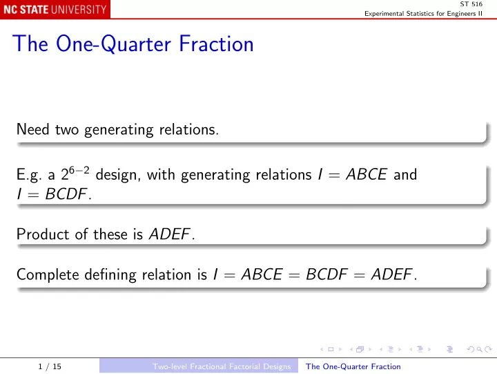
ST 516 Experimental Statistics for Engineers II The One-Quarter Fraction Need two generating relations. E.g. a 2 6 − 2 design, with generating relations I = ABCE and I = BCDF . Product of these is ADEF . Complete defining relation is I = ABCE = BCDF = ADEF . 1 / 15 Two-level Fractional Factorial Designs The One-Quarter Fraction

ST 516 Experimental Statistics for Engineers II This is a resolution-IV design. Why? There is no resolution-V 2 6 − 2 design. Why not? To set up runs, either: create the full 2 6 design with ABCE and BCDF confounded with blocks, and choose the block with both positive; or set up a basic design in 4 factors, then add the other 2. For example, basic design is 2 4 in A , B , C , D , and defining relations show that E = ABC and F = BCD . 2 / 15 Two-level Fractional Factorial Designs The One-Quarter Fraction

ST 516 Experimental Statistics for Engineers II Basic Design Run A B C D E = ABC F = BCD 1 - - - - - - 2 + - - - + - 3 - + - - + + 4 + + - - - + 5 - - + - + + 6 + - + - - + 7 - + + - - - 8 + + + - + - 9 - - - + - + 10 + - - + + + 11 - + - + + - 12 + + - + - - . . . . . . . . . . . . . . . . . . . . . 16 + + + + + + 3 / 15 Two-level Fractional Factorial Designs The One-Quarter Fraction

ST 516 Experimental Statistics for Engineers II Projections This 2 6 − 2 design projects into: IV a single complete replicate of a 2 4 design in A , B , C , and D , and any other of the 12 subsets of 4 factors that is not a word in the defining relation; a replicated one-half fraction of a 2 4 design in A , B , C , and E , and in the other two subsets of 4 factors that are a word in the defining relation; two replicates of a 2 3 design in any three factors; four replicates of a 2 2 design in any two factors. 4 / 15 Two-level Fractional Factorial Designs The One-Quarter Fraction

ST 516 Experimental Statistics for Engineers II Example with this design Response is shrinkage in injection molding, and factors are: A , mold temperature; B , screw speed; C , holding time; D , cycle time; E , gate size; F , hold pressure. 5 / 15 Two-level Fractional Factorial Designs The One-Quarter Fraction

ST 516 Experimental Statistics for Engineers II Data file injection.txt: A B C D E F Shrinkage - - - - - - 6 + - - - + - 10 - + - - + + 32 + + - - - + 60 - - + - + + 4 + - + - - + 15 - + + - - - 26 + + + - + - 60 - - - + - + 8 + - - + + + 12 - + - + + - 34 + + - + - - 60 - - + + + - 16 + - + + - - 5 - + + + - + 37 + + + + + + 52 6 / 15 Two-level Fractional Factorial Designs The One-Quarter Fraction

ST 516 Experimental Statistics for Engineers II R commands injection <- read.table("data/injection.txt", header = TRUE) for (j in 1:(ncol(injection) - 1)) injection[ , j] <- coded(injection[ , j]) summary(lm(Shrinkage ~ A * B * C * D * E * F, injection)) Output Call: lm(formula = Shrinkage ~ A * B * C * D * E * F, data = injection) Residuals: ALL 16 residuals are 0: no residual degrees of freedom! Coefficients: (48 not defined because of singularities) Estimate Std. Error t value Pr(>|t|) (Intercept) 27.3125 NA NA NA A 6.9375 NA NA NA B 17.8125 NA NA NA C -0.4375 NA NA NA D 0.6875 NA NA NA 7 / 15 Two-level Fractional Factorial Designs The One-Quarter Fraction

ST 516 Experimental Statistics for Engineers II Output, continued E 0.1875 NA NA NA F 0.1875 NA NA NA A:B 5.9375 NA NA NA A:C -0.8125 NA NA NA B:C -0.9375 NA NA NA A:D -2.6875 NA NA NA B:D -0.0625 NA NA NA C:D -0.0625 NA NA NA D:E 0.3125 NA NA NA A:B:D 0.0625 NA NA NA A:C:D -2.4375 NA NA NA Residual standard error: NaN on 0 degrees of freedom Multiple R-Squared: 1, Adjusted R-squared: NaN F-statistic: NaN on 15 and 0 DF, p-value: NA Note that all 2-factor interactions are aliased with one or two other 2-factor interactions, and all but two 3-factor interactions are aliased with main effects or other 3-factor interactions. 8 / 15 Two-level Fractional Factorial Designs The One-Quarter Fraction

ST 516 Experimental Statistics for Engineers II Main effect alias chains A = BCE = DEF = ABCDF B = ACE = CDF = ABDEF C = ABE = BDF = ACDEF D = BCF = AEF = ABCDE E = ABC = ADF = BCDEF F = BCD = ADE = ABCEF 9 / 15 Two-level Fractional Factorial Designs The One-Quarter Fraction

ST 516 Experimental Statistics for Engineers II Other alias chains AB = CE = ACDF = BDEF AC = BE = ABDF = CDEF AD = EF = BCDE = ABCF AE = BC = DF = ABCDEF AF = DE = ABCD = BCEF BD = CF = ACDE = ABEF BF = CD = ACEF = ABDE ABD = CDE = ACF = BEF ACD = BDE = ABF = CEF 10 / 15 Two-level Fractional Factorial Designs The One-Quarter Fraction

ST 516 Experimental Statistics for Engineers II 70 ● B 60 50 40 Effects 30 A ● A:B ● 20 10 ● ● ● ● ● ● ● ● ● ● ● ● 0 0.0 0.5 1.0 1.5 Half Normal plot 11 / 15 Two-level Fractional Factorial Designs The One-Quarter Fraction

ST 516 Experimental Statistics for Engineers II The half-normal plot suggests that A and B are the important effects. Interaction plot with(injection, interaction.plot(A, B, Shrinkage)) Residual plots suggest that C is a dispersion effect. Analyze absolute residuals r <- residuals(aov(Shrinkage ~ A * B, injection)) summary(aov(abs(r) ~ A * B * C * D * E * F, injection)) 12 / 15 Two-level Fractional Factorial Designs The One-Quarter Fraction

ST 516 Experimental Statistics for Engineers II Output Df Sum Sq Mean Sq A 1 1.00 1.00 B 1 0.25 0.25 C 1 56.25 56.25 D 1 3.06 3.06 E 1 1.00 1.00 F 1 1.00 1.00 A:B 1 0.25 0.25 A:C 1 2.25 2.25 B:C 1 1.00 1.00 A:D 1 1.56 1.56 B:D 1 0.06 0.06 C:D 1 2.25 2.25 D:E 1 9.00 9.00 A:B:D 1 0.56 0.56 A:C:D 1 0.25 0.25 13 / 15 Two-level Fractional Factorial Designs The One-Quarter Fraction

ST 516 Experimental Statistics for Engineers II Montgomery suggests calculating, for each effect, F ∗ = log sum of squares of residuals at high level sum of squares of residuals at low level In R, not easy to calculate F ∗ , but we can look at the half-normal plot for abs( r ) or r 2 : qqnorm(aov(abs(r) ~ A * B * C * D * E * F, injection), label = TRUE) qqnorm(aov(r^2 ~ A * B * C * D * E * F, injection), label = TRUE) The effects shown in the second of these, for r^2 , are essentially sum of squares of residuals at high level − sum of squares of residuals at low level 14 / 15 Two-level Fractional Factorial Designs The One-Quarter Fraction

ST 516 Experimental Statistics for Engineers II In the spirit of R’s “Scale-Location” residual plot, we could use � | residual | : qqnorm(aov(sqrt(abs(r)) ~ A * B * C * D * E * F, injection)) � All three half-normal plots ( r 2 , | r | , and | r | ) give the same indication as F ∗ : C appears to be a dispersion factor. 15 / 15 Two-level Fractional Factorial Designs The One-Quarter Fraction