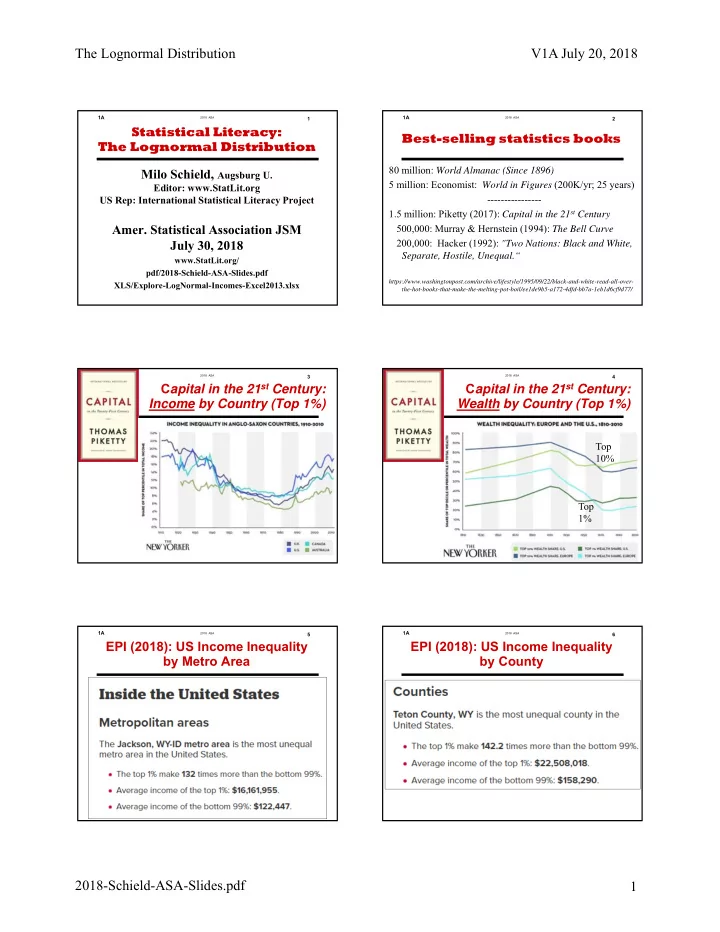
The Lognormal Distribution V1A July 20, 2018 1A 1A 2018 ASA 1 - PDF document

The Lognormal Distribution V1A July 20, 2018 1A 1A 2018 ASA 1 2018 ASA 2 Statistical Literacy: Best-selling statistics books The Lognormal Distribution 80 million: World Almanac (Since 1896) Milo Schield, Augsburg U. 5 million: Economist: World in Figures (200K/yr; 25 years) Editor: www.StatLit.org ---------------- US Rep: International Statistical Literacy Project 1.5 million: Piketty (2017): Capital in the 21 st Century Amer. Statistical Association JSM 500,000: Murray & Hernstein (1994): The Bell Curve 200,000: Hacker (1992): "Two Nations: Black and White, July 30, 2018 Separate, Hostile, Unequal.“ www.StatLit.org/ pdf/2018-Schield-ASA-Slides.pdf https://www.washingtonpost.com/archive/lifestyle/1995/09/22/black-and-white-read-all-over- XLS/Explore-LogNormal-Incomes-Excel2013.xlsx the-hot-books-that-make-the-melting-pot-boil/ee1de9b5-a172-4dfd-bb7a-1eb1d6cf9d77/ 1A 1A 2018 ASA 3 2018 ASA 4 C apital in the 21 st Century: C apital in the 21 st Century: Income by Country (Top 1%) Wealth by Country (Top 1%) . . Top 10% Top 1% 1A 1A 2018 ASA 5 2018 ASA 6 EPI (2018): US Income Inequality EPI (2018): US Income Inequality by Metro Area by County . . 2018-Schield-ASA-Slides.pdf 1

The Lognormal Distribution V1A July 20, 2018 1A 1A 2018 ASA 7 2018 ASA 8 Piketty: Piketty: C apital in the 21 st Century Censored Data Problem The key property of Pareto distributions is this: Evaluate income share held by top 1% over time. the “ratio of ‘average income y*(y) of individuals Data source: Tax data with income above y’ to y does not depend on the Problem: Tax authorities censors high-income data. income threshold y.” So, how did Piketty deduce the income share of top 1% [Ave Income > y] / y = Beta “if β = 2, the average income of individuals with Piketty used a model: the Pareto distribution. income above $100,000 is $200,000 and the By fitting this model to uncensored incomes, he inferred average income of individuals with income above the distribution of the censored incomes. $1 million is $2 million.” Atkinson et al (2011). P 12-14. Atkinson, Piketty, Suan (2011). P 12-14. 1A 1A 2018 ASA 9 2018 ASA 10 EPI (2018): Income Inequality Bibliography Top 1% Since 1920 by Country . . 1A 1A 2018 ASA 11 2018 ASA 12 Log-Normal Distribution . . Log-Normal shape is common. Examples: • Incomes (bottom 97%), assets, size of cities • Weight and blood pressure of humans (by gender) • Stock and portfolio returns Log-Normal is useful. • Function is easier to work with than a histogram • Understand what determines or explains shape • calculate the share of total income held by the top X% • calculate share of total income held by the ‘above-average’ • explore effects of change in mean-median ratio. 2018-Schield-ASA-Slides.pdf 2

The Lognormal Distribution V1A July 20, 2018 1A 1A 2018 ASA 13 2018 ASA 14 Log-Normal Distribution: Log-Normal Atchison and Brown Distribution of Units “In many ways, it [the Log-Normal] has remained the . Theoretical Distribution of Units by Income Cinderella of distributions, the interest of writers in the Mode: 20K learned journals being curiously sporadic and that of the 100% Cumulative Distribution Function (CDF): authors of statistical text-books but faintly aroused.” Percentage of Units with Incomes below price 75% “We … state our belief that the lognormal is as fundamental a 50% distribution in statistics as is the normal, despite the stigma of Units can be individuals, households or families the derivative nature of its name.” 25% Probability Distribution Function (PDF): as a percentage of the Modal PDF Shape is determined by the mean-median ratio. 0% 0 50 100 150 200 250 300 350 400 450 500 Aitchison and Brown (1957). P 1. Incomes ($1,000) LogNormal Dist of Units Median=50K; Mean=80K 1A 1A 2018 ASA 15 2018 ASA 16 Distribution of Households Paired Distributions and Total Income by Income For anything that is distributed by X, there are If the distribution of households by income is log- always two distributions: normal with normal parameters mu# and sigma#, 1. Distribution of subjects by X the distribution of total income by household 2. Distribution of total X by X. income has a log-normal distribution where Sometime we ignore the 2 nd : height or weight. mu$ = mu# + sigma#^2; sigma$ = sigma#. Sometimes we care about the 2 nd : income or assets. See Aitchison and Brown (1957), p. 158. Special thanks to Mohammod Irfan (Denver University) for his help on this topic. Surprise: If the 1 st is lognormal, so is the 2 nd . 1A 1A 2018 ASA 17 2018 ASA 18 Distribution of Distribution of Total Income Households and Total Income Distribution of Total Income . Distribution of Households by Income; by Income per Household Distribution of Total Income by Amount Mode: 50K 100% 100% Distribution of Total Income by Median: Amount of Income Percentage of Maximum 128K 75% Mode: $50K 75% Cumulative Distribution Function (CDF): Median: $128K Percentage of Total Income below price Ave $205K 50% 50% Probability Distribution Function (PDF): 25% Households by Income 25% as a percentage of the Modal PDF Mode: $20K; Median: $50K Mean=$80K 0% 0% 0 50 100 150 200 250 300 350 400 450 500 0 50 100 150 200 Income ($1,000) Unit Incomes ($1,000) Log Normal Distribution of Households by Income Income/House: Mean=80K; Median=50K LogNormal Dist of Units by Income Median=50K; Mean=80K 2018-Schield-ASA-Slides.pdf 3

The Lognormal Distribution V1A July 20, 2018 1A 1A 2018 ASA 19 2018 ASA 20 Lorenz Curve and Champagne-Glass Gini Coefficient Distribution Pctg of Households vs. Pctg of Income Pctg of Income vs. Pctg. of Households . The Gini coefficient 100% 100% is determined by the Top 50% (above $50k): 83% of total Income Top 10% (above $175k: 38% of total Income Bottom‐Up 80% 80% Mean#/Median# ratio. Top 1% (above $475k): 8.7% of total Income Gini = 0.507 Percentage of Income Percentage of Households Top 0.1% (above $1M): 1.7% of total Income 60% 60% The bigger this ratio 40% 40% Gini Coefficient: the bigger the Gini Top 50% (above $50k) have 83% of total Income 0.507 Top 10% (above $175k) have 38% of total Income 20% 20% Top 1% (above $475k) have 8.7% of total Income Bigger means coefficient and the Top 0.1% (above $1M) have 1.7% of total Income more unequal greater the economic 0% 0% 0% 20% 40% 60% 80% 100% 0% 20% 40% 60% 80% 100% inequality. Percentage of Income Percentage of Households Log Normal Distribution of Households by Income Income/House: Mean=80K; Median=50K Log Normal Distribution of Households by Income Income/House: Mean=80K; Median=50K 1A 1A 2018 ASA 21 2018 ASA 22 As Mean-Median Ratio  Atchison-Brown Rich get Richer (relatively) Balance Theorem Log-normal distribution. Median HH income: $50K. If the average household income is located at the X th percentile, then it follows that; Top 5% Top 1% Mean# Min$ %Income Min$ %Income Gini • X% of all HH have incomes below the average income 55 103 11% 138 2.9% 0.24 (1-X)% of all HH are located above this point 60 135 15% 204 4.2% 0.33 65 165 18% 270 5.5% 0.39 • X% of all HH income is earned by Households above this point. 70 193 20% 337 6.6% 0.44 75 220 23% 406 7.7% 0.48 • Above-average income households earn X/(1-X) times 80 246 25% 477 8.7% 0.51 their pro-rata share of total income 85 272 27% 549 9.7% 0.53 • Below-average income households earn (1-X)/X times 90 298 29% 623 10.7% 0.56 their pro-rata share of income. 1A 1A 2018 ASA 23 2018 ASA 24 What Causes an Increase in Conclusion the Mean-Median Ratio? Bad things : Crony capitalism, illegal gains. Using the LogNormal distribution provides a simple, principled way for students Good things: • to explore a plausible distribution of incomes More people getting college degrees. • to understand the factors that influence the change Creating ways to do existing things better, cheaper or in income distributions faster (Making pins, . Providing value or entertainment that people enjoy. Creating ways to do new things that were not doable before (telegraph, telephone, internet). 2018-Schield-ASA-Slides.pdf 4

1A 2018 ASA 1 Statistical Literacy: The Lognormal Distribution Milo Schield, Augsburg U. Editor: www.StatLit.org US Rep: International Statistical Literacy Project Amer. Statistical Association JSM July 30, 2018 www.StatLit.org/ pdf/2018-Schield-ASA-Slides.pdf XLS/Explore-LogNormal-Incomes-Excel2013.xlsx

1A 2018 ASA 2 Best-selling statistics books 80 million: World Almanac (Since 1896) 5 million: Economist: World in Figures (200K/yr; 25 years) ---------------- 1.5 million: Piketty (2017): Capital in the 21 st Century 500,000: Murray & Hernstein (1994): The Bell Curve 200,000: Hacker (1992): "Two Nations: Black and White, Separate, Hostile, Unequal.“ https://www.washingtonpost.com/archive/lifestyle/1995/09/22/black-and-white-read-all-over- the-hot-books-that-make-the-melting-pot-boil/ee1de9b5-a172-4dfd-bb7a-1eb1d6cf9d77/

1A 2018 ASA 3 C apital in the 21 st Century: Income by Country (Top 1%) .

1A 2018 ASA 4 C apital in the 21 st Century: Wealth by Country (Top 1%) . Top 10% Top 1%

1A 2018 ASA 5 EPI (2018): US Income Inequality by Metro Area .

1A 2018 ASA 6 EPI (2018): US Income Inequality by County .