The Interplay of Information Theory, Probability, and Statistics - - PowerPoint PPT Presentation

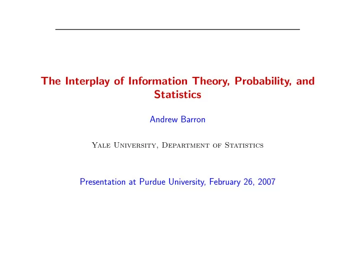
The Interplay of Information Theory, Probability, and Statistics

Andrew Barron

Yale University, Department of Statistics

Presentation at Purdue University, February 26, 2007

Outline

• Information Theory Quantities and Tools *

Entropy, relative entropy Shannon and Fisher information Information capacity

• Interplay with Statistics **

Information capacity determines fundamental rates for parameter estimation and function estimation

• Interplay with Probability Theory

Central limit theorem *** Large deviation probability exponents **** for Markov chain Monte Carlo and optimization

* Cover & Thomas, Elements of Information Theory, 1990 ** Hengartner & Barron 1998 Ann.Stat; Yang & Barron 1999 Ann.Stat. *** Barron 1986 Ann.Prob; Johnson & B. 2004 Ann.Prob; Madiman & B. 2006 ISIT **** Csiszar 1984 Ann.Prob.

Outline for Information and Probability

• Central Limit Theorem

If X1, X2, . . . , Xn are i.i.d. with mean zero and variance 1 and fn is the density function of (X1 + X2 + . . . + Xn)/√n and φ is the standard normal density, then D(fn||φ) ց 0 if and only if this entropy distance is ever finite

• Large Deviations and Markov Chains

If {Xt} is i.i.d. or reversible Markov and f is bounded then there is an exponent Dǫ characterized as a relative entropy with which P{1 n

n

• t=1

f(Xt) ≥ E[f] + ǫ} ≤ e−nDǫ Markov chains based on local moves permit a differential equation which when solved determines the exponent Dǫ Should permit determination of which chains provide accurate Monte Carlo estimates.

Entropy

• For a random variable Y or sequence Y = (Y1, Y2, . . . , YN)

with probability mass or density function p(y), the Shannon entropy is H(Y ) = E log 1 p(Y )

• It is the shortest expected codelength for Y
• It is the exponent of the size of the smallest set that has

most of the probability

Relative Entropy

• For distributions PY , QY the relative entropy or information divergence

is D(PY ||QY ) = EP

• log p(Y )

q(Y )

• It is non-negative: D(P||Q) ≥ 0 with equality iff P = Q
• It is the redundancy, the expected excess of the codelength log 1/q(Y )

beyond the optimal log 1/p(Y ) when Y ∼ P

• It is the drop in wealth exponent when gambling according to Q on
• utcomes distributed according to P
• It is the exponent of the smallest Q measure set that has most of the P

probability (the exponent of probability of error of the best test): Chernoff

• It is a standard measure of statistical loss for function estimation with

normal errors and other statistical models (Kullback, Stein) D(θ∗||θ) = D(PY |θ∗||PY |θ)

Statistics Basics

• Data:

Y = (Y1, Y2, . . . , Yn)

• Likelihood:

p(Y |θ) = p(Y1|θ) · p(Y2|θ) · · · p(Yn|θ)

• Maximum Likelihood Estimator (MLE):

ˆ θ = arg max

θ

p(Y |θ)

• Same as

arg minθ log

1 p(Y |θ)

• MLE Consistency Wald 1948

ˆ θ = arg min

θ

1 n

n

• i=1

log p(Yi|θ∗) p(Yi|θ) = arg min

θ

ˆ Dn(θ∗||θ) Now ˆ Dn(θ∗||θ) → D(θ∗||θ) as n → ∞ and D(θ∗||ˆ θn) → 0

• Efficiency in smooth families: ˆ

θn is asymptotically Normal(θ, (nI(θ))−1)

• Fisher information:

I(θ) = E[▽ log p(Y |θ) ▽T log p(Y |θ)]

Statistics Basics

• Data:

Y = Y n = (Y1, Y2, . . . , Yn)

• Likelihood: p(Y |θ),

θ ∈ Θ

• Prior:

p(θ) = w(θ)

• Marginal:

p(Y ) =

• p(Y |θ)w(θ)dθ

Bayes mixture

• Posterior:

p(θ|Y ) = w(θ)p(Y |θ)/p(Y )

• Parameter loss function: ℓ(θ, ˆ

θ), for instance squared error (θ − ˆ θ)2

• Bayes parameter estimator: ˆ

θ achieves minˆ

θ E[ℓ(θ, ˆ

θ)|Y ] ˆ θ = E[θ|Y ] =

• θp(θ|Y )dθ
• Density loss function ℓ(P, Q), for instance D(P, Q)
• Bayes density estimator: ˆ

p(y) = p(y|Y ) achives minQ E[ℓ(P, Q)|Y ] ˆ p(y) =

• p(y|θ)p(θ|Y n)dθ
• Predictive coherence: Bayes estimator is the predictive density p(Yn+1|Y n)

evaluated at Yn+1 = y

• Other loss functions do not share this property

Chain Rules for Entropy and Relative Entropy

• For joint densities

p(Y1, Y2, . . . , YN) = p(Y1) p(Y2|Y1) · · · p(YN|YN−1, . . . , Y1)

• Taking the expectation this is

H(Y1, Y2, . . . YN) = H(Y1) + H(Y2|Y1) + . . . + H(YN|YN−1, . . . , Y1)

• The joint entropy grows like HN for stationary processes
• For the relative entropy between distributions for a string Y = Y N =

(Y1, . . . , YN) we have the chain rule D(PY ||QY ) =

• n

EPD(PYn+1|Y n||QYn+1|Y n)

• Thus the total divergence is a sum of contributions in which the predictive

distributions QYn+1|Y n based on the previous n data points is measured for their quality of fit to PYn+1|Y n for each n less than N

• With good predictive distributions we can arrange D(PY N||QY N) to grow

at rates slower than N simultaneously for various P

Tying data compression to statistical learning

• Various plug-in ˆ

pn(y) = p(y|ˆ θn) and Bayes predictive estimators ˆ pn(y) = q(y|Y n) =

• p(y|θ)p(θ|Y n)dθ

achieve individual risk D(PY |θ|| ˆ Pn) ∼ c n ideally with asymptotic constant c = d/2 where d is the parameter di- mension (more on that ideal constant later)

• Successively evaluating the predictive densities q(Yn+1|Y n) these piece

fit together to give a joint density q(Y N) with total divergence D(PY N|θ||QY N) ∼ c log N

• Conversely from any coding distribution QY N with good redundancy

D(PY N|θ)||QY N) a succession of predictive estimators can be obtained

• Similar conclusions hold for nonparametric function estimation problems

Local Information, Estimation, and Efficiency

• The Fisher information I(θ) = IFisher(θ) arises naturally in local analysis
• f Shannon information and related statistics problems.
• In smooth families the relative entropy loss is locally a squared error

D(θ||ˆ θ) ∼ 1 2(θ − ˆ θ)TI(θ)(θ − ˆ θ)

• Efficient estimates have asymptotic covariance not more than I(θ)−1
• If smaller than that at some θ the estimator is said to be superefficient
• The expectation of the asymptotic distribution for the right side above is

d 2n

• The set of parameter values with smaller asymptotic covariance is negli-

gible, in the sense that it has zero measure

Efficiency of Estimation via Info Theory Analysis

• LeCam 1950s: Efficiency of Bayes and maximum likelihood estimators.

Negligibility of superefficiency for bounded loss and any efficient estimator

• Hengartner and B. 1998: Negligibility of superefficiency for any parameter

estimator using ED(θ||ˆ θ) and any density estimator using ED(P|| ˆ Pn)

• The set of parameter values for which nED(PY |θ|| ˆ

Pn) has limit not smaller than d/2 includes all but a negligible set of θ

• The proof does not require a Fisher information, yet correspond to the

classical conclusion when there is such

• The efficient level is from coarse covering properties of Euclidean space
• The core of the proof is the chain rule plus a result of Rissanen
• Rissanen 1986: no choice of joint distribution achieves D(PY N|θ||QYN)

better than (d/2) log N except in a negligible set of θ

• The proof works also for nonparametric problems
• Negligibility of superefficiency determined by sparsity of its cover

Mutual Information and Information Capacity

• We shall need two additional quantities in our discussion of

information theory and statistics. These are: the Shannon mutual information I and the information capacity C

Shannon Mutual Information

• For a family of distributions PY |U of a random variable Y given an input

U distributed according to PU, the Shannon mutual information is I(Y ; U) = D(PU,Y ||PUPY ) = EUD(PY |U||PY )

• In communications, it is the rate, the exponent of the number of input

strings U that can be reliably communicated across a channel PY |U

• It is the error probability exponent with which a random U erroneously

passes the test of being jointly distributed with a received string Y

• In data compression, I(Y ; θ) is the Bayes average redundancy of the code

based on the mixture PY when θ = U is unknown

• In a game with relative entropy loss, it is the Bayes optimal value corre-

sponding to the the Bayes mixture PY being the choice of QY achieving I(Y ; θ) = min

QY EθD(PY |θ||QY )

• Thus it is the average divergence from the centroid PY

Information Capacity

• For a family of distributions PY |U the Shannon information capacity is

C = max

PU I(Y ; U)

• It is the communications capacity, the maximum rate that can be reliably

communicated across the channel

• In the relative entropy game it is the maximin value

C = max

Pθ

min

QY EPθD(PY |θ||QY )

• Accordingly it is also the minimax value

C = min

QY max θ

D(PY |θ||QY )

• Also known as the information radius of the family PY |θ
• In data compression, this means that C = maxPθ I(Y ; θ) is also the

minimax redundancy for the family PY |θ (Gallager; Ryabko; Davisson)

• In recent years the information capacity has been shown to also answer

questions in statistics as we shall discuss

Information Asymptotics for Bayes Procedures

• The Bayes mixture density p(Y ) =
• p(Y |θ)w(θ)dθ satisfies in smooth

parametric families the Laplace approximation log 1 p(Y ) = log 1 p(Y |ˆ θ) + d 2 log N 2π + log |I(ˆ θ)|1/2 w(ˆ θ) + op(1)

• Underlies Bayes and description length criteria for model selection
• Clarke & B. 1990 show for θ in the interior of the parameter space that

D(PY |θ||PY ) = d 2 log N 2πe + log |I(θ)|1/2 w(θ) + o(1)

• Likewise, via Clarke & B. 1994, the average with respect to the prior has

IShannon(Y ; θ) = d 2 log N 2πe +

• w(θ) log |IFisher(θ)|1/2

w(θ) + o(1)

• Provides capacity of multi-antenna systems (d input, N output) as well

as minimax asymptotics for data compression and statistical estimation

Minimax Asymptotics in Parametric Families

• We identify the form of prior w(θ) that equalizes the risk D(PY |θ||PY )

and maximizes the Bayes risk I(Y ; θ). This prior should be proportional to |IFisher(θ)|1/2, known in statistics and physics as Jeffreys’ prior.

• This prior gives equal weight to small equal-radius relative entropy balls
• Clark and B. 1994: on any compact K in the interior of Θ, the informa-

tion capacity CN (and minimax redundancy) satisfies CN = d 2 log N 2πe + log

• K

|IFisher(θ)|1/2dθ + o(1)

• Asymptotically maximin priors and corresponding asymptotically minimax

procedure are obtained by using boundary modifications of Jeffreys’ prior

• Xie and B. 1998, 1999: refinement applicable to the whole probability

simplex in the case of finite alphabet distributions

• Liang and B. 2004 show exact minimaxity for finite sample size in families

with group structure such as location & scale problems, conditional on initial observations to make the minimax answer finite

Minimax Asymptotics for Function Estimation

• Let F be a function class and let data Y with sample size n come

independently from a distribution PY |f with f ∈ F

• Thus f can be a density function, a regression function, a discriminant

function or an intensity function depending in the nature of the model

• Let F be endowed with a metric d(f, g) such as L2 or Hellinger distance
• The Kolmogorov metric entropy or ǫ−entropy, denoted H(ǫ) is the log
• f the size of the smallest cover of F by finitely many functions, such

that every f in F is within ǫ of one of the functions in the cover

• The metric entropy rate is obtained by matching

H(ǫn) n = ǫ2

n

• The minimax rate of function estimation is

rn = min

ˆ fn

max

f∈F Ed2(f, ˆ

fn)

• The information capacity rate of {PY |f, f ∈ F} is

Cn = 1 n sup

Pf

I(Y ; f)

Minimax Asymptotics for Function Estimation

• Suppose D(PY |f||PY |g) is equivalent to the squared metric d2(f, g) in F

in that their ratio is bounded above and below by positive constants

• Theorem: (Yang & B. 1998) The minimax rate of function estimation,

the metric entropy rate, and the information capacity rate are the same rn ∼ Cn ∼ ǫ2

n

• The proof in one direction uses the chain rule and bounds the cumulative

risk of a Bayes procedure using the uniform prior on an optimal cover

• The other direction is based on use of Fano’s inequality
• Typical function classes constrain the smoothness s of the function, e.g.

s may be number of bounded derivatives, and have H(ǫ) ∼ (1/ǫ)1/s

• Accordingly

rn ∼ ǫ2

n ∼ n−2s/(2s+1)

• Analogous results in Haussler and Opper 1997.
• Precursors were in work by Pinsker, by Hasminskii, and by Birge

Outline for Information and Probability

• Central Limit Theorem

If X1, X2, . . . , Xn are i.i.d. with mean zero and variance 1 and fn is the density function of (X1 + X2 + . . . + Xn)/√n and φ is the standard normal density, then D(fn||φ) ց 0 if and only if this entropy distance is ever finite

• Large Deviations and Markov Chains

If {Xt} is i.i.d. or reversible Markov and f is bounded then there is an exponent Dǫ characterized as a relative entropy with which P{1 n

n

• t=1

f(Xt) ≥ E[f] + ǫ} ≤ e−nDǫ Markov chains based on local moves permit a differential equation which when solved provides approximately the exponent Dǫ. Should permit determination of which chains provide accurate Monte Carlo estimates.

Outline for Information and CLT

• Entropy and the Central Limit Problem
• Entropy Power Inequality (EPI)
• Monotonicity of Entropy and new subset sum EPI
• Variance Drop Lemma
• Projection and Fisher Information
• Rates of Convergence in the CLT

Entropy Basics

• For a mean zero random variable X with density f(x) and finite variance

σ2 = 1, the differential entropy is H(X) = E[log

1 f(X)]

the entropy power of X is e2H(X)/2πe

• For a Normal(0, σ2) random variable Z, with density function φ,

the differential entropy is H(Z) = (1/2) log(2πeσ2) the entropy power of Z is σ2

• The relative entropy is D(f||φ) =
• f(x) log f(x)

φ(x)dx

it is non-negative: D(f||φ) ≥ 0 with equality iff f = φ it is larger than (1/2)||f − φ||2

1

Maximum entropy property Boltzmann, Jaynes, Shannon

Let Z be a normal random variable with the same mean and variance as a random variable X, then H(X) ≤ H(Z) with equality iff X is normal The relative entropy quantifies the entropy gap H(Z) − H(X) = D(f||φ)

Maximum entropy property Boltzmann, Jaynes, Shannon

Let Z be a normal random variable with the same mean and variance as a random variable X, then H(X) ≤ H(Z) with equality iff X is normal. The relative entropy quantifies the entropy gap. Indeed, this is Kullback’s proof of the maximum entropy property H(Z) − H(X) =

• φ(x) log

1 φ(x)dx −

• f(x) log

1 f(x)dx =

• f(x) log

1 φ(x)dx −

• f(x) log

1 f(x)dx =

• f(x) log f(x)

φ(x)dx = D(f||φ) ≥ 0 Here log

1 φ(x) = x2 2σ2 log e+ 1 2 log 2πσ2 is quadratic in x, so both f and φ give

it the same expectation, which is 1

2 log 2πeσ2.

Fisher Information Basics

• For a mean zero random variable X with differentiable density f(x) and

finite variance σ2 = 1, the score function is score(X) = d

dx log f(x)

the Fisher information is I(X) = E[score2(X)].

• For a Normal(0, σ2) random variable Z, with density function φ,

the score function is linear score(Z) = −Z/σ2 the Fisher information is I(Z) = 1/σ2

• The relative Fisher information is J(f||φ) =
• f(x)
• d

dx log f(x) φ(x)

2 dx it is non-negative it is larger than D(f||φ)

• Minimum Fisher info property (Cramer-Rao ineq): I(X) ≥ 1/σ2

equality iff Normal

• The information gap satisfies: I(X) − I(Z) = J(f||φ)

The Central Limit Problem

For independent identically distributed random variables X1, X2, . . . , Xn, with E[X] = 0 and V AR[X] = σ2 = 1, consider the standardized sum X1 + X2 + . . . + Xn √n . Let its density function be fn and its distribution function Fn. Let the standard normal density be φ and its distribution function Φ. Natural questions:

• In what sense do we have convergence to the normal?
• Do we come closer to the normal with each step?
• Can we give clean bounds on the “distance” from the normal and a

corresponding rate of convergence?

Convergence

• In distribution: Fn(x) → Φ(x)

Classical via Fourier methods or expansions of expectations of smooth functions. Linnick 59, Brown 82 via info measures applied to smoothed distributions.

• In density: fn(x) → φ(x)

Prohorov 52 showed ||fn − φ||1 → 0 iff fn exists eventually. Kolmogorov & Gnedenko 54 ||fn − φ||∞ → 0 iff fn bounded eventually.

• In Shannon Information: H( 1

√n

n

i=1 Xi) → H(Z)

Barron 86 shows D(fn||φ) → 0 iff it is eventually finite.

• In Fisher Information: I( 1

√n

n

i=1 Xi) → 1/σ2

Johnson & Barron 04 shows J(fn||φ) → 0 iff it is eventually finite.

Original Entropy Power Inequality

Shannon 48, Stam 59: For independent random variables with densities,

e2H(X1+X2) ≥ e2H(X1) + e2H(X2)

where equality holds if and only if the Xi are normal. Also e2H(X1+...+Xn) ≥

n

• j=1

e2H(Xj)

Original Entropy Power Inequality

Shannon 48, Stam 59: For independent random variables with densities,

e2H(X1+X2) ≥ e2H(X1) + e2H(X2)

where equality holds if and only if the Xi are normal. Central Limit Theorem Implication For Xi i.i.d., let Hn = H 1 √n

n

• i=1

Xi

• nHn is superadditive

Hn1+n2 ≥ n1 n1 + n2 Hn1 + n2 n1 + n2 Hn2

• monotonicity for doubling sample size

H2n ≥ Hn

• The superadditivity of nHn and the monotonicity for the powers of two

subsequence are key in the proof of entropy convergence [Barron ’86]

Leave-one-out Entropy Power Inequality

Artstein, Ball, Barthe and Naor 2004 (ABBN): For independent Xi e2H(X1+...+Xn) ≥ 1 n − 1

n

• i=1

e2H

j=i Xj

• Remarks
• This strengthens the original EPI of Shannon and Stam.
• ABBN’s proof is elaborate.
• Our proof (Madiman & Barron 2006) uses familiar and simple tools and

proves a more general result, that we present.

• The leave-one-out EPI implies in the iid case that entropy is increasing:

Hn ≥ Hn−1

• A related proof of monotonicity is developed contemporaneously in Tulino

& Verd´ u 2006.

• Combining with Barron 1986 the monotonicity implies

Hn ր H(Normal) and Dn =

• fn log fn

φ ց 0

New Entropy Power Inequality

Subset-sum EPI (Madiman and Barron) For any collection S of subsets s of indices {1, 2, . . . , n}, e2H(X1+...+Xn) ≥ 1 r(S)

• s∈S

e2H(sums) where sums =

j∈s Xj is the subset-sum

r(S) is the prevalence, the maximum number of subsets in S in which any index i can appear Examples

• S=singletons,

r(S) = 1,

• riginal EPI
• S=leave-one-out sets,

r(S) = n–1, ABBN’s EPI

• S=sets of size m,

r(S) = n–1

m–1

• ,

leave n–m out EPI

• S=sets of m consecutive indices,

r(S) = m

New Entropy Power Inequality

Subset-sum EPI For any collection S of subsets s of indices {1, 2, . . . , n}, e2H(X1+...+Xn) ≥ 1 r(S)

• s∈S

e2H(sums) Discriminating and balanced collections S

• Discriminating if for any i, j, there is a set in S containing i but not j
• Balanced if each index i appears in the same number r(S) of sets in S

Equality in the Subset-sum EPI For discriminating and balanced S, equality holds in the subset-sum EPI if and only if the Xi are normal

In this case, it becomes

n

• i=1

ai = 1 r(S)

• s∈S
• i∈s

ai with ai = Var(Xi)

New Entropy Power Inequality

Subset-sum EPI For any collection S of subsets s of indices {1, 2, . . . , n}, e2H(X1+...+Xn) ≥ 1 r(S)

• s∈S

e2H(sums) CLT Implication Let Xi be independent, but not necessarily identically distributed. The entropy of variance-standardized sums increases “on average”: H sumtotal σtotal

• ≥
• s∈S

λs H sums σs

• where
• σ2

total is the variance of sumtotal = n i=1 Xi and σ2 s is the variance of sums = j∈s Xj

• The weights

λs =

σ2

s

r(S)σ2

total

are proportional to σ2

s

• The weights add to 1 for balanced collections S

New Fisher Information Inequality

For independent X1, X2, . . . , Xn with differentiable densities, 1 I(sumtotal) ≥ 1 r(S)

• s∈S

1 I(sums) Remarks

• This extends Fisher information inequalities of Stam and ABBN
• Recall from Stam ’59

1 I(X1 + . . . + Xn) ≥ 1 I(X1) + . . . + 1 I(Xn)

• For discriminating and balanced S, equality holds iff the Xi are normal

New Fisher Information Inequality

For independent X1, X2, . . . , Xn with differentiable densities, 1 I(sumtotal) ≥ 1 r(S)

• s∈S

1 I(sums) CLT Implication

• For i.i.d. Xi , let In = I

1 √n

n

• i=1

Xi

• The Fisher information In is a decreasing sequence:

In ≤ In−1

[ABBN ’04]

Combining with Johnson and Barron ’04 implies In ց I(Normal) and J(fn||φ) ց 0

• For i.n.i.d. Xi, the Fisher info. of standardized sums decreases on average

I sumtotal σtotal

• ≤
• s∈S

λs I sums σs

The Link between H and I

Definitions

• Shannon entropy:

H(X) = E

• log

1 f(X)

• Score function:

score(X) = ∂

∂x log f(X)

• Fisher information:

I(X) = E [ score2(X) ] Relationship For a standard normal Z independent of X,

• Differential version:

d dtH(X + √ tZ) = 1 2I(X + √ tZ)

[de Bruijn, see Stam ’59]

• Integrated version:

H(X) = 1 2 log(2πe) − 1 2 ∞

• I(X +

√ tZ) − 1 1 + t

• dt

[Barron ’86]

The Projection Tool

For each subset s, score(sumtotal) = E

• score(sums)
• sumtotal
• Hence, for weights ws that sum to 1,

score(sumtotal) = E

s∈S

ws score(sums)

• sumtotal
• Pythagorean inequality

The Fisher info. of the sum is the mean squared length of the projection

✚✚✚✚✚✚✚✚✚✚✚✚✚ ✚

score(sumtotal) ws score(sums) I(sumtotal) ≤ E

s∈S

ws score(sums) 2

The Heart of the Matter

Recall the Pythagorean inequality I(sumtotal) ≤ E

s∈S

ws score(sums) 2 and apply the variance drop lemma to get I(sumtotal) ≤ r(S)

• s∈S

w2

sI(sums)

The Variance Drop Lemma

Let X1, X2, . . . , Xn be independent. Let Xs = (Xi : i ∈ s) and gs(Xs) be some mean-zero function of Xs. Then sums of such functions g(X1, X2, . . . , Xn) =

• s∈S

gs(Xs) have the variance bound Eg2 ≤ r(S)

• s∈S

Eg2

s(Xs)

The Variance Drop Lemma

Let X1, X2, . . . , Xn be independent. Let Xs = (Xi : i ∈ s) and gs(Xs) be some mean-zero function of Xs. Then sums of such functions g(X1, X2, . . . , Xn) =

• s∈S

gs(Xs) have the variance bound Eg2 ≤ r(S)

• s∈S

Eg2

s(Xs)

Remarks

• Note that r(S) ≤ |S|, hence the “variance drop”
• Examples:

S=singletons has r = 1 : additivity of variance with independent summands S=leave-one-out sets has r = n−1 as in the study of the jackknife and U-statistics

• Proof is based on ANOVA decomposition

[Hoeffding ’48, Efron and Stein ’81]

• Introduced in leave-one-out case to info. inequality analysis by ABBN ’04

Optimized Form for I

We have, for all weights ws that sum to 1, I(sumtotal) ≤ r(S)

• s∈S

w2

sI(sums)

Optimizing over w yields the new Fisher information inequality 1 I(sumtotal) ≥ 1 r(S)

• s∈S

1 I(sums)

Optimized Form for H

We have (again) I(sumtotal) ≤ r(S)

• s∈S

w2

sI(sums)

Equivalently, I(sumtotal) ≤

• s∈S

wsI

• sums
• r(S)ws
• Adding independent normals and integrating,

H(sumtotal) ≥

• s∈S

wsH

• sums
• r(S)ws
• Optimizing over w yields the new Entropy Power Inequality

e2H(sumtotal) ≥ 1 r(S)

• s∈S

e2H(sums)

Fisher information and M.M.S.E. Estimation

Model: Y = X + Z where Z ∼ N(0, 1) and X is to be estimated

• Optimal estimate:

ˆ X = E[X|Y ] Fact: score(Y ) = ˆ X–Y Note: X– ˆ X and ˆ X–Y are orthogonal, and sum to –Z Hence: I(Y ) = E( ˆ X–Y )2 = 1–E(X– ˆ X)2 = 1 − Minimal M.S.E. From L.D. Brown ’70’s [c.f. the text of Lehmann and Casella ’98]

• Thus derivative of entropy can be expressed equivalently in terms of either

I(Y ) or minimal M.S.E.

• Guo, Shamai and Verd´

u, 2005 use the minimal M.S.E. interpretation to give a related proof of the EPI and Tulino and Verd´ u 2006 use this M.S.E. interpretation to give a related proof of monotonicity in the CLT

Recap: Subset-sum EPI

For any collection S of subsets s of indices {1, 2, . . . , n}, e2H(sumtotal) ≥ 1 r(S)

• s∈S

e2H(sums)

• Generalizes original EPI and ABBN’s EPI
• Simple proof using familiar tools
• Equality holds for normal random variables

Comment on CLT rate bounds

For iid Xi let Jn = J(fn||φ) and Dn = D(fn||φ) Suppose the distribution of the Xi has a finite Poincar´ e constant R. Using the pythagorean identity for score projection, Johnson & Barron ’04 show: Jn ≤ 2R n J1 Dn ≤ 2R n D1

• Implies a 1/√n rate of convergence in distribution, known to hold for

random variables with non-zero finite third moment.

• Our finite Poincar´

e assumption implies finite moments of all orders.

• Do similar bounds on information distance hold assuming only finite initial

information distance and finite third moment?

Summary

Two ingredients

• score of sum = projection of scores of subset-sums
• variance drop lemma

yield the conclusions

• existing Fisher information and entropy power inequalities
• new such inequalities for arbitrary collections of subset-sums
• monotonicity of I and H in central limit theorems

refinements using the pythagorean identity for the score projection yield

• convergence in information to the Normal
• order 1/n bounds on information distance from the Normal
• − ◦ − ◦