Estimation Theory Overview Introduction Up until now we have - PowerPoint PPT Presentation
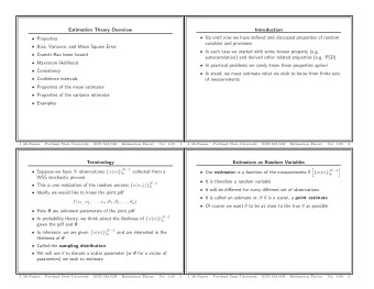
Estimation Theory Overview Introduction Up until now we have defined and discussed properties of random Properties variables and processes Bias, Variance, and Mean Square Error In each case we started with some known property (e.g.
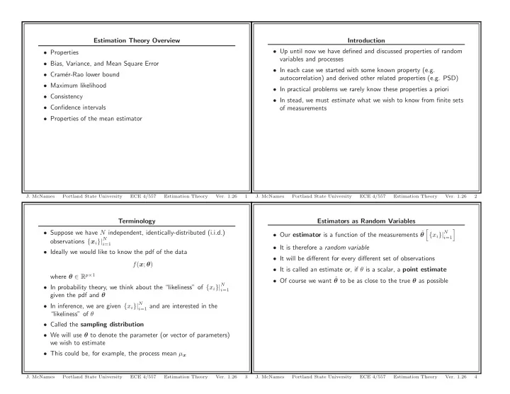
Estimation Theory Overview Introduction • Up until now we have defined and discussed properties of random • Properties variables and processes • Bias, Variance, and Mean Square Error • In each case we started with some known property (e.g. • Cram´ er-Rao lower bound autocorrelation) and derived other related properties (e.g. PSD) • Maximum likelihood • In practical problems we rarely know these properties a priori • Consistency • In stead, we must estimate what we wish to know from finite sets • Confidence intervals of measurements • Properties of the mean estimator J. McNames Portland State University ECE 4/557 Estimation Theory Ver. 1.26 1 J. McNames Portland State University ECE 4/557 Estimation Theory Ver. 1.26 2 Terminology Estimators as Random Variables � � • Suppose we have N independent, identically-distributed (i.i.d.) • Our estimator is a function of the measurements ˆ { x i }| N θ i =1 observations { x i }| N i =1 • It is therefore a random variable • Ideally we would like to know the pdf of the data • It will be different for every different set of observations f ( x ; θ ) • It is called an estimate or, if θ is a scalar, a point estimate where θ ∈ R p × 1 • Of course we want ˆ θ to be as close to the true θ as possible • In probability theory, we think about the “likeliness” of { x i }| N i =1 given the pdf and θ • In inference, we are given { x i }| N i =1 and are interested in the “likeliness” of θ • Called the sampling distribution • We will use θ to denote the parameter (or vector of parameters) we wish to estimate • This could be, for example, the process mean µ x J. McNames Portland State University ECE 4/557 Estimation Theory Ver. 1.26 3 J. McNames Portland State University ECE 4/557 Estimation Theory Ver. 1.26 4
Natural Estimators Good Estimators N � � = 1 � µ x = ˆ { x i }| N ˆ θ x i θ (ˆ f ˆ θ ) i =1 N n =1 • This is the obvious or “natural” estimator of the process mean ˆ θ • Sometimes called the average or sample mean θ • It will also turn out to be the “best” estimator • Without loss of generality, let us consider a scalar parameter θ for • I will define “best” shortly the time being • What is a “good” estimator N – Distribution of ˆ � � θ should be centered at the true value = 1 � x = ˆ { x i }| N µ x ) 2 σ 2 ˆ θ ( x i − ˆ i =1 N – Want the distribution to be as narrow as possible n =1 • Lower-order moments enable coarse measurements of “good” • This is the obvious or “natural” estimator of the process variance • Not the “best” J. McNames Portland State University ECE 4/557 Estimation Theory Ver. 1.26 5 J. McNames Portland State University ECE 4/557 Estimation Theory Ver. 1.26 6 Bias Variance Bias of an estimator ˆ Variance of an estimator ˆ θ of a parameter θ is defined as θ of a parameter θ is defined as �� 2 � B (ˆ θ ) � E[ˆ �� � θ ] − θ var(ˆ � ˆ ˆ θ ) = σ 2 � � θ � E θ − E θ ˆ � • Unbiased : an estimator is said to be unbiased if B (ˆ θ ) = 0 • A measure of the spread of ˆ θ about its mean • This implies the pdf of the estimator is centered at the true value θ • Would like the variance to be as small as possible • The sample mean is unbiased • The estimator of variance on the earlier slide is biased • Unbiased estimators are generally good, but they are not always best (more later) J. McNames Portland State University ECE 4/557 Estimation Theory Ver. 1.26 7 J. McNames Portland State University ECE 4/557 Estimation Theory Ver. 1.26 8
Bias-Variance Tradeoff The Bias-Variance Tradeoff θ (ˆ θ (ˆ f ˆ θ ) f ˆ θ ) θ (ˆ θ (ˆ f ˆ θ ) f ˆ θ ) ˆ ˆ θ θ θ θ ˆ ˆ θ θ θ θ • Understanding of the bias-variance tradeoff is crucial to this course • In many cases minimizing variance conflicts with minimizing bias • Unbiased models are not always best • Note that ˆ θ � 0 has zero variance, but is generally biased • The methods we will use to estimate the model coefficients are biased • In these cases we must trade variance for bias (or vice versa) • But they may be more accurate, because they have less variance • This idea applies to nonlinear models as well J. McNames Portland State University ECE 4/557 Estimation Theory Ver. 1.26 9 J. McNames Portland State University ECE 4/557 Estimation Theory Ver. 1.26 10 Bias, Variance, and Modeling Notation and Prediction Error y = g ( x ) + ε g = g ( x ) g = ˆ ˆ g ( x ) g e = E[ˆ ˆ g ( x )] y ( x ) = g ( x ) + ε • Expectation is taken over the distribution of data sets used to y ( x ) = ˆ ˆ g ( x ) construct ˆ g ( x ) and the distribution of the process noise f ( ε ) • In the modeling context, we are usually interested in estimating a • Everything is a function of x function • Recall that ε is i.i.d. with zero mean • For a given input x , this function is a scalar • We are treating x as a fixed, non-random variable • We can define θ = g ( x ) • The dependence on x is not shown to simplify notation • Thus, all of the ideas that apply to estimating parameters also The prediction error for a new, given input is defined as apply to estimating functional relationships g ) 2 ] PE( x ) = E[( y − ˆ g ) + ε ) 2 ] = E[(( g − ˆ g ) 2 ] + 2 E[( g − ˆ g ) ε ] + E[ ε 2 ] = E[( g − ˆ MSE( x ) + σ 2 = ε J. McNames Portland State University ECE 4/557 Estimation Theory Ver. 1.26 11 J. McNames Portland State University ECE 4/557 Estimation Theory Ver. 1.26 12
The Bias-Variance Tradeoff Derivation Bias-Variance Tradeoff Derivation Continued 1 y = g ( x ) + ε g = g ( x ) g = ˆ ˆ g ( x ) ˆ g e = E[ˆ g ( x )] g e ) 2 − 2( g − ˆ ① = E[( g − ˆ g e )(ˆ g − ˆ g e )] E[ g 2 − 2 g ˆ g 2 g 2 g 2 = g e + ˆ e − 2 g (ˆ g − ˆ g e )] + 2ˆ e − 2ˆ e E[ g 2 − 2 g ˆ g 2 = g e + ˆ e − 2 g ˆ g + 2 g ˆ g e ] • Only ˆ g is a random function E[ g 2 − 2 g ˆ g 2 = g + ˆ e ] • Nothing else is dependent on the data set g 2 − 2 g E[ˆ g 2 = g ] + ˆ e g 2 − 2 g ˆ g ) 2 ] g 2 MSE( x ) = E[( g − ˆ = g e + ˆ e g e ) } 2 ] g e ) 2 = ( g − ˆ = E[ { ( g − ˆ g e ) − (ˆ g − ˆ ⎡ ⎤ Thus g e ) 2 − 2( g − ˆ g e ) 2 = E ⎣ ( g − ˆ g e )(ˆ g − ˆ g e ) + (ˆ g − ˆ ⎦ � �� � � �� � MSE( x ) = ① + ② ① ② g e ) 2 + E[(ˆ g e ) 2 ] = ( g − ˆ g − ˆ g ]) 2 + E � g ]) 2 � = ( g − E[ˆ (ˆ g − E[ˆ J. McNames Portland State University ECE 4/557 Estimation Theory Ver. 1.26 13 J. McNames Portland State University ECE 4/557 Estimation Theory Ver. 1.26 14 Bias-Variance Tradeoff Comments Bias-Variance Tradeoff Comments Continued g ]) 2 + E g ]) 2 + E � g ]) 2 � � g ]) 2 � MSE( x ) = ( g − E[ˆ (ˆ g − E[ˆ MSE( x ) = ( g − E[ˆ (ˆ g − E[ˆ = Bias 2 + Variance = Bias 2 + Variance • Large variance: the model is sensitive to small changes in the • Large variance, small bias data set – If the model is too flexible, it can overfit the data • Large bias: if the model was compared to the true function on a – The model will change dramatically from one data set to large number of data sets, the expected value of the model ˆ g ( x ) another would not be close to the true function g ( x ) – In this case it has high variance, but potentially low variance • If the model is sensitive to small changes in the data, a biased • Small variance, large bias model may have smaller error ( MSE ) than an unbiased model – If the model is not very flexible, it may not capture the true relationship between the inputs and the output • If the data is strongly collinear, biased models can result in more accurate models! – It will not vary as much from one data set to another – In this case the model has low variance, but potentially high bias J. McNames Portland State University ECE 4/557 Estimation Theory Ver. 1.26 15 J. McNames Portland State University ECE 4/557 Estimation Theory Ver. 1.26 16
Recommend
More recommend
Explore More Topics
Stay informed with curated content and fresh updates.
