Estimation Theory Overview Introduction Up until now we have - PowerPoint PPT Presentation
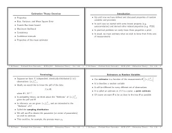
Estimation Theory Overview Introduction Up until now we have defined and discussed properties of random Properties variables and processes Bias, Variance, and Mean Square Error In each case we started with some known property (e.g.
Estimation Theory Overview Introduction • Up until now we have defined and discussed properties of random • Properties variables and processes • Bias, Variance, and Mean Square Error • In each case we started with some known property (e.g. • Cram´ er-Rao lower bound autocorrelation) and derived other related properties (e.g. PSD) • Maximum likelihood • In practical problems we rarely know these properties apriori • Consistency • In stead, we must estimate what we wish to know from finite sets • Confidence intervals of measurements • Properties of the mean estimator • Properties of the variance estimator • Examples J. McNames Portland State University ECE 538/638 Estimation Theory Ver. 1.09 1 J. McNames Portland State University ECE 538/638 Estimation Theory Ver. 1.09 2 Terminology Estimators as Random Variables • Suppose we have N observations { x ( n ) }| N − 1 � � • Our estimator is a function of the measurements ˆ { x ( n ) }| N − 1 collected from a θ 0 0 WSS stochastic process • It is therefore a random variable • This is one realization of the random process { x ( n, ζ ) } N − 1 0 • It will be different for every different set of observations • Ideally we would like to know the joint pdf • It is called an estimate or, if θ is a scalar, a point estimate f ( x 1 , x 2 , . . . , x n ; θ 1 , θ 2 , . . . , θ p ) • Of course we want ˆ θ to be as close to the true θ as possible • Here θ are unknown parameters of the joint pdf • In probability theory, we think about the likeliness of { x ( n ) }| N − 1 0 given the pdf and θ • In inference, we are given { x ( n ) }| N − 1 and are interested in the 0 likeliness of θ • Called the sampling distribution • We will use θ to denote a scalar parameter (or θ for a vector of parameters) we wish to estimate J. McNames Portland State University ECE 538/638 Estimation Theory Ver. 1.09 3 J. McNames Portland State University ECE 538/638 Estimation Theory Ver. 1.09 4
Natural Estimators Good Estimators N − 1 = 1 � � µ x = ˆ { x ( n ) }| N − 1 � ˆ θ x ( n ) θ (ˆ f ˆ θ ) 0 N n =0 ˆ • This is the obvious or “natural” estimator of the process mean θ θ • Sometimes called the average or sample mean • What is a “good” estimator? • It will also turn out to be the “best” estimator – Distribution of ˆ θ should be centered at the true value • I will define “best” shortly – Want the distribution to be as narrow as possible N − 1 = 1 � � • Lower-order moments enable coarse measurements of “goodness” x = ˆ { x ( n ) }| N − 1 µ x ] 2 σ 2 � ˆ θ [ x ( n ) − ˆ 0 N n =0 • This is the obvious or “natural” estimator of the process variance • Not the “best” J. McNames Portland State University ECE 538/638 Estimation Theory Ver. 1.09 5 J. McNames Portland State University ECE 538/638 Estimation Theory Ver. 1.09 6 Bias Variance Bias of an estimator ˆ Variance of an estimator ˆ θ of a parameter θ is defined as θ of a parameter θ is defined as B (ˆ θ ) � E[ˆ �� 2 � θ ] − θ � var(ˆ � ˆ θ − E[ˆ θ ) = σ 2 θ � E θ ] � � ˆ � Normalized Bias of an estimator ˆ θ of a non-negative parameter θ is Normalized Standard deviation of an estimator ˆ defined as θ of a non-negative ε b � B (ˆ θ ) parameter θ is defined as ε r � σ ˆ θ θ θ • Unbiased : an estimator is said to be unbiased if B (ˆ θ ) = 0 • A measure of the spread of ˆ θ about its mean • This implies the pdf of the estimator is centered at the true value θ • Would like the variance to be as small as possible • The sample mean is unbiased • The estimator of variance on the earlier slide is biased • Unbiased estimators are generally good, but they are not always best (more later) J. McNames Portland State University ECE 538/638 Estimation Theory Ver. 1.09 7 J. McNames Portland State University ECE 538/638 Estimation Theory Ver. 1.09 8
Bias-Variance Tradeoff Mean Square Error Mean Square Error of an estimator ˆ θ of a parameter θ is defined as θ (ˆ θ (ˆ f ˆ θ ) f ˆ θ ) � θ − θ | 2 � | ˆ θ + | B (ˆ MSE( θ ) � E = σ 2 θ ) | 2 ˆ Normalized MSE of an estimator ˆ θ of a parameter θ is defined as ˆ ˆ θ θ θ θ ε � MSE(ˆ θ ) θ � = 0 • In many cases minimizing variance conflicts with minimizing bias θ • Note that ˆ θ � 0 has zero variance, but is generally biased • The decomposition of MSE into variance plus bias squared is very • In these cases we must trade variance for bias (or vice versa) similar to the DC and AC decomposition of signal power • We will use MSE as a global measure of estimator performance • Note that two different estimators may have the same MSE , but different bias and variance • This criterion is convenient for building estimators • Creating a problem we can solve J. McNames Portland State University ECE 538/638 Estimation Theory Ver. 1.09 9 J. McNames Portland State University ECE 538/638 Estimation Theory Ver. 1.09 10 Cram´ er-Rao Lower Bound Cram´ er-Rao Lower Bound Comments 1 1 1 1 var(ˆ var(ˆ θ ) ≥ − � 2 � = − θ ) ≥ � 2 � = − ∂ 2 ln f x ; θ ( x ; θ ) �� � � ∂ 2 ln f x ; θ ( x ; θ ) �� � � ∂ ln f x ; θ ( x ; θ ) E ∂ ln f x ; θ ( x ; θ ) E E E ∂θ 2 ∂θ 2 ∂θ ∂θ • Minimum Variance Unbiased (MVU) : Estimators that are both • Efficient Estimator : an unbiased estimate that achieves the unbiased and have the smallest variance of all possible estimators CRLB with equality • Note that these do not necessarily achieve the minimum MSE • If it exists, then the unique solution is given by • Cram´ er-Rao Lower Bound (CRLB) is a lower bound on ∂ ln f x ; θ ( x ; θ ) = 0 unbiased estimators ∂θ • Derived in text where the pdf is evaluated at the observed outcome x ( ζ ) • Log Likelihood Function of θ is ln f x ; θ ( x ; θ ) • Maximum Likelihood (ML) Estimate : an estimator that • Note that the pdf f x ; θ ( x ; θ ) describes the distribution of the data satisfies the equation above (stochastic process), not the parameter • This can be generalized to vectors of parameters • Recall that θ is not a random variable, it is a parameter that • Limited use — f x ; θ ( x ; θ ) is rarely known in practice defines the distribution J. McNames Portland State University ECE 538/638 Estimation Theory Ver. 1.09 11 J. McNames Portland State University ECE 538/638 Estimation Theory Ver. 1.09 12
Consistency Confidence Intervals • Confidence Interval : interval, a ≤ θ ≤ b , that has a specified • Consistent Estimator an estimator such that probability of covering the unknown true parameter value N →∞ MSE(ˆ lim θ ) = 0 Pr { a < θ ≤ b } = 1 − α • Implies the following as the sample size grows ( N → ∞ ) • The interval is estimated from the data, therefore it is also a pair – The estimator becomes unbiased of random variables – The variance approaches zero • Confidence Level : coverage probability of a confidence interval, – The distribution f ˆ θ ( x ) becomes an impulse centered at θ 1 − α • The confidence interval is not uniquely defined by the confidence level • More later J. McNames Portland State University ECE 538/638 Estimation Theory Ver. 1.09 13 J. McNames Portland State University ECE 538/638 Estimation Theory Ver. 1.09 14 Properties of the Sample Mean Sample Mean Confidence Intervals N − 1 � ˆ µ x � 1 � � 2 � � 1 − 1 µ x − µ x ˆ x ( n ) f ˆ µ x (ˆ µ x ) = √ √ exp √ N 2 2 π ( σ x / N ) σ x / N n =0 E[ˆ µ x ] = µ x N N µ x ) = 1 � 1 − | ℓ | � γ x ( ℓ ) ≤ 1 � � � µ x − k σ x µ x < µ x + k σ x � var(ˆ γ x ( ℓ ) Pr √ < ˆ √ = N N N N N ℓ = − N ℓ = − N � µ x − k σ x µ x + k σ x � Pr ˆ √ < µ x < ˆ √ = 1 − α µ x ) = σ 2 • If x ( n ) is WN, then this reduces to var(ˆ x N N N • The estimator is unbiased • In general, we don’t know the pdf • If γ x ( ℓ ) → 0 as ℓ → ∞ , then var(ˆ µ x ) → 0 (estimator is • If we can assume the process is Gaussian and IID, we know the consistent) pdf (sampling distribution) of the estimator • The variance increases as the correlation of x ( n ) increases • If N is large and the distribution doesn’t have heavy tails, the • In processes with long memory or heavy tails, it is harder to distribution of ˆ µ x is Gaussian by the Central Limit Theorem (CLT) estimate the mean J. McNames Portland State University ECE 538/638 Estimation Theory Ver. 1.09 15 J. McNames Portland State University ECE 538/638 Estimation Theory Ver. 1.09 16
Recommend
More recommend
Explore More Topics
Stay informed with curated content and fresh updates.
