State estimation approach to nonstationary Introduction inverse - PowerPoint PPT Presentation

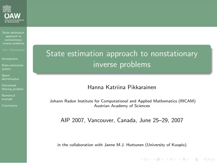
State estimation approach to nonstationary inverse problems H.K. Pikkarainen State estimation approach to nonstationary Introduction inverse problems State estimation system Space discretization Discretized Hanna Katriina Pikkarainen filtering problem Numerical example Johann Radon Institute for Computational and Applied Mathematics (RICAM) Austrian Academy of Sciences Conclusions AIP 2007, Vancouver, Canada, June 25–29, 2007 in the collaboration with Janne M.J. Huttunen (University of Kuopio)

Overview State estimation approach to nonstationary inverse problems Introduction 1 H.K. Pikkarainen Introduction State estimation State estimation system 2 system Space discretization Space discretization 3 Discretized filtering problem Numerical example Discretized filtering problem 4 Conclusions Numerical example 5 Conclusions 6

Overview State estimation approach to nonstationary inverse problems Introduction 1 H.K. Pikkarainen Introduction State estimation State estimation system 2 system Space discretization Space discretization 3 Discretized filtering problem Numerical example Discretized filtering problem 4 Conclusions Numerical example 5 Conclusions 6

Dynamical inverse problem State estimation approach to nonstationary inverse problems H.K. Pikkarainen we are interested in the quantity X in a domain along time Introduction a model for the time evolution of X State estimation system the evolution model may not be correct Space = ⇒ an additional source term representing possible modelling discretization errors Discretized filtering problem no direct measurements of X Numerical example the quantity Y depends linearly on X Conclusions = ⇒ observe the quantity Y at direct time instants an additional measurement noise in the measured values of Y calculate an estimate for X based on the measured values of Y

Overview State estimation approach to nonstationary inverse problems Introduction 1 H.K. Pikkarainen Introduction State estimation State estimation system 2 system Space discretization Space discretization 3 Discretized filtering problem Numerical example Discretized filtering problem 4 Conclusions Numerical example 5 Conclusions 6

State evolution equation State estimation approach to nonstationary inverse problems D ⊂ R d is a domain that corresponds to the object of interest H.K. Pikkarainen X = X ( t , x ) , x ∈ D , is the unknown distribution of the physical Introduction quantity we are interested in at time t ≥ 0 State estimation system A : D ( A ) ⊂ L 2 ( D ) → L 2 ( D ) is defined by Space discretization d d Discretized filtering problem � � f �→ a ij ∂ i ∂ j f + b i ∂ i f + cf (1) Numerical i , j =1 i =1 example Conclusions where � d � �  � � f ∈ H 2 ( D ) :  D ( A ) = β i ∂ i f + γ f = 0 (2)   ∂ D i =1

State evolution equation State estimation approach to nonstationary inverse problems H.K. Pikkarainen Assumption Introduction Let x 0 ∈ L 2 ( D ) , Γ 0 and Q be positive self-adjoint trace class State estimation operators from L 2 ( D ) to itself with trivial null spaces, and T > 0 . system Space discretization According to Kolmogorov’s existence theorem there exist Discretized filtering problem a probability space (Ω , F , P ) , Numerical a Q -Wiener process W ( t ) , t ∈ [0 , T ] , with values in L 2 ( D ) , example Conclusions an L 2 ( D ) -valued random variable X 0 such that X 0 and W ( t ) are independent for all t ∈ (0 , T ] , X 0 is Gaussian with mean x 0 and covariance Γ 0 .

State evolution equation State estimation approach to nonstationary inverse problems H.K. Pikkarainen We assume that the time evolution of the process X can be modelled Introduction by the stochastic partial differential equation State estimation system Space d X ( t ) = AX ( t )d t + d W ( t ) (3) discretization Discretized filtering problem for every t > 0 with the initial value Numerical example X (0) = X 0 . (4) Conclusions The term d W ( t ) is a source term representing possible modelling errors in the time evolution model.

Observation equation State estimation approach to nonstationary inverse problems H.K. Pikkarainen Introduction The measurement process is modelled by the equation State estimation system Space Y ( t ) = C ( t ) X ( t ) + S ( t ) (5) discretization Discretized filtering problem for all 0 < t ≤ T where { C ( t ) } t ∈ (0 , T ] is a family of bounded linear operators from L 2 ( D ) to R L and S ( t ) , t ∈ [0 , T ] , is an R L -valued Numerical example stochastic process. The process S represents possible measurement Conclusions errors.

Time discrete state estimation system State estimation approach to nonstationary inverse problems H.K. Pikkarainen the measurements are made in time instants Introduction State estimation 0 < t 1 < . . . < t n ≤ T system we use the notation Space discretization Discretized t 0 := 0 , ∆ k +1 := t k +1 − t k , (6) filtering problem Numerical X k +1 := X ( t k +1 ) , Y k +1 := Y ( t k +1 ) , (7) example Conclusions C k := C ( t k ) , S k +1 := S ( t k +1 ) (8) for all k = 0 , . . . , n − 1

Time discrete state estimation system State estimation approach to nonstationary inverse problems The time discrete state estimation system is H.K. Pikkarainen Introduction X k +1 = U (∆ k +1 ) X k + W k +1 , k = 0 , . . . , n − 1 , (9) State estimation system Y k = C k X k + S k , k = 1 , . . . , n (10) Space discretization where the state noise W k +1 is given by the formula Discretized filtering problem � t k +1 Numerical example W k +1 = U ( t k +1 − s ) d W ( s ) . (11) Conclusions t k By the Riesz representation theorem there exist such functions ϕ ( k ) ∈ L 2 ( D ) that ( C k f ) p = ( f , ϕ ( k ) p ) for all f ∈ L 2 ( D ) , k = 1 . . . , n p and p = 1 , . . . , L .

Overview State estimation approach to nonstationary inverse problems Introduction 1 H.K. Pikkarainen Introduction State estimation State estimation system 2 system Space discretization Space discretization 3 Discretized filtering problem Numerical example Discretized filtering problem 4 Conclusions Numerical example 5 Conclusions 6

Space discretization State estimation approach to nonstationary inverse problems Definition H.K. Pikkarainen Introduction The sequence { V m } ∞ m =1 of finite-dimensional subspaces of L 2 ( D ) is State estimation called a sequence of appropriate discretization spaces if system Space (i) V m ⊂ V m +1 for all m ∈ N , discretization Discretized (ii) ∪ V m = L 2 ( D ) . filtering problem Numerical example { V m } ∞ m =1 is a sequence of appropriate discretization spaces in Conclusions L 2 ( D ) l } N m { ψ m l =1 is an orthonormal basis of V m for all m ∈ N Z m := (( Z , ψ m N m )) T is the discretized 1 ) , ( Z , ψ m 2 ) . . . , ( Z , ψ m version of a random variable Z at the discretization level m

Discretized state estimation system State estimation approach to nonstationary inverse problems H.K. Pikkarainen By using the time discrete state estimation equation (9)–(10) we are Introduction able to give a state estimation system for the finite-dimensional State estimation processes { X m k } n k =0 and { Y k } n k =1 . The discretized state estimation system system is Space discretization Discretized X m k +1 = A m k +1 X m k + ǫ m k +1 + W m k +1 , k = 0 , . . . , n − 1 , (12) filtering problem Numerical Y k = C m k X m k + ν m k + S k , k = 1 , . . . , n . (13) example Conclusions The matrices A m k +1 and C m are given by k j , ϕ ( k ) ( A m k ) ij := ( U (∆ k ) ψ m j , ψ m i ) and ( C m k ) pj := ( ψ m p ) for all i , j = 1 , . . . , N m , k = 1 , . . . , n and p = 1 , . . . , L .

Discretization errors State estimation approach to nonstationary inverse problems The discrete stochastic process H.K. Pikkarainen ǫ m k +1 := (( X k , ( I − P m ) U ∗ (∆ k ) ψ m 1 ) , . . . , Introduction State estimation . . . , ( X k , ( I − P m ) U ∗ (∆ k ) ψ m N m )) T (14) system Space discretization represent the discretization error in the state evolution equation, Discretized filtering problem W m = (( W k , ψ m 1 ) , . . . , ( W k , ψ m N m )) T (15) Numerical k example Conclusions is the state noise vector and k := (( X k , ( I − P m ) ϕ ( k ) 1 ) , . . . , ( X k , ( I − P m ) ϕ ( k ) ν m L )) T (16) represents the discretization error in the observation equation for all k = 1 , . . . , n .

Overview State estimation approach to nonstationary inverse problems Introduction 1 H.K. Pikkarainen Introduction State estimation State estimation system 2 system Space discretization Space discretization 3 Discretized filtering problem Numerical example Discretized filtering problem 4 Conclusions Numerical example 5 Conclusions 6