Modelling covariance kernels for nonstationary random fields - PowerPoint PPT Presentation
Modelling covariance kernels for nonstationary random fields Christopher G. Small University of Waterloo University of Guelph, October 2007 0-0 1. Random fields and covariance kernels 2. The role of covariance kernels in semiparametric
Modelling covariance kernels for nonstationary random fields Christopher G. Small University of Waterloo University of Guelph, October 2007 0-0
1. Random fields and covariance kernels 2. The role of covariance kernels in semiparametric inference 3. The Karhunen-Lo` eve expansion 4. The estimation problem reconsidered 5. An application 1
1. Random fields and covariance kernels 2
� For a random sample, inference about the mean µ of the � Moreover, heteroscedasticity is a problem for the optimal variates depends upon knowledge or estimation of the variance σ 2 . In practice the variance is harder to estimate than the mean. � For a random field X ( t ), inference about the mean function estimation of µ . To optimally estimate µ we must model or estimate the variance function. � When Γ is unknown we need to estimate it. What methods are µ ( t ) requires knowledge or estimation of the covariance kernel Γ( s , t ) = Cov[ X ( s ) , X ( t ) ]. available when the process is not second order stationary, i.e. , when Γ( s , t ) � = γ ( s − t )? 3
� By a random field we shall mean a family of random � In practice, we only observe a finite “piece” of this random variables X ( t ) indexed by some parameter t ∈ R q . � When R is a countable set—finite or denumerable, usually a field. So we shall assume that t lies in some bounded subset R of R q . � When R is an open subset of R q then X ( t ) is said to be a lattice—then we say that X ( t ) is a discrete random field . continuous random field . 4
Stochastic processes X ( t ) , t ≥ 0 are random fields .... 5
Example: Lynx Pelt Prices, HBC 1857-1911. Elton & Nicholson (1942). 6
140 120 100 80 60 40 20 0 1850 1860 1870 1880 1890 1900 1910 1920 7
Random sets are also special cases where X ( t ) ∈ { 0 , 1 } .... 8
Example: Two-dimensional random set. Integrated circuit data, Mallory et al. (1983). 9
20 18 16 14 12 10 8 6 4 2 2 4 6 8 10 12 14 16 18 20 22 24 10
2. Role of covariance kernels in semiparametric inference 11
� Let E [ X ( t )] = µ θ ( t ) and Cov[ X ( s ) , X ( t )] = Γ θ ( s , t ) � Both µ θ and Γ θ are assumed to be known real-valued functions be the mean function and covariance kernel respectively, where s , t ∈ R and θ ∈ R k . of the unknown parameter θ ∈ R k . 12
� With these semiparametric assumptions, θ can be estimated by a linear functional estimating equation of the form L ( X ; � θ ) = 0 where � L ( X ; θ ) = [ X ( t ) − µ θ ( t )] d A θ ( t ) , R where A θ is a vector-valued measure on R taking values in R k . 13
� For a discrete random field where t typically lies in a lattice, this reduces to an estimating function of the form � For a continuous random field , typically d A θ ( t ) = a θ ( t ) d t , � L ( X ; θ ) = a θ ( t ) [ X ( t ) − µ θ ( t )] . t ∈R � In both cases, a θ : R q → R k is a vector-valued coefficient so that � L ( X ; θ ) = a θ ( t ) [ X ( t ) − µ θ ( t )] d t . � In this talk, we will emphasize the continuous case. However, R function which is functionally independent of X . most remarks apply with appropriate modification to other types of random fields. 14
� The optimal estimating function is that which has a vector-valued measure A θ satisfying � Γ θ ( s , t ) d A θ ( s ) = ˙ µ θ ( t ) . R where ˙ µ θ ( t ) is the vector-valued partial derivative of µ θ ( t ) with respect to θ . 15
� Problem 1. Note that the equation for A θ must be solved for There are two problems with implementing this optimal solution: each value of the parameter θ , iteratively used within any algorithm that solves the equation L ( � θ ) = 0 . – For example, when θ ∈ R 2 , a discrete random field on a 20 × 20 lattice requiring as little as ten iterations over θ , � Problem 2. In practice, we do not know Γ θ . This must will need the solution to 800 simultaneous non-sparse linear equations, ten successive times in a row, just to produce a single approximation to � θ . usually be estimated as well!! 16
3. The Karhunen-Lo` eve expansion 17
� The solution to both of these problems can be obtained using � Let b 1 ( t ) , b 2 ( t ) , . . . be the set of eigenfunctions for the the Karhunen-Lo` eve expansion . kernel Γ satisfying � b j ( s )Γ( s , t ) d s = σ 2 j b j ( t ) R for j = 1 , 2 , . . . . Here, the parameter θ is suppressed in the � Since Γ is positive definite, the eigenvalues will be also be notation for simplicity. Since Γ is symmetric, the eigenfunctions b j can be chosen to be real and � Provided that the kernel function Γ is complete , the set of orthonormal . positive. So we can write the j th eigenvalue as σ 2 j . standardised eigenfunctions of Γ will form an orthonormal basis for L 2 ([ R ]). 18
� Using the completeness condition, we may write � ∞ X ( t ) = Y j b j ( t ) , j =1 where Y 1 , Y 2 , . . . satisfy � Let E ( Y j ) = µ j for all j . � � We have Var( Y j ) = σ 2 Y j = X ( t ) b j ( t ) d t . R � We will also need j . � ∞ µ ( t ) = ˙ µ j b j ( t ) ˙ j =1 � ˙ where ˙ µ j = µ ( t ) b j ( t ) d t . 19
� Writing out X in terms of the Karhunen-Lo` eve expansion, we obtain an equivalent expression for L ( θ ), namely � ∞ σ − 2 L ( θ ) = j ( θ ) ˙ µ j ( θ ) [ Y j ( θ ) − µ j ( θ )] , j =1 which is a rather standard looking quasi-likelihood equation , with the exception that the random variables Y j are also functions of the parameter θ . 20
4. The estimation problem reconsidered 21
� We need only sum the first few terms of the K.-L. expansion. Proposed solution to Problem 1: � Instead, choose Y ∗ Since � j σ 2 j < ∞ , we choose terms with the most significant leading eigenvalues. Say, the first m terms. j = Y j ( θ ∗ ), where θ ∗ is some simple consistent approximation to θ —possibly, but not necessarily an estimator. However, consider θ ∗ as fixed, not random. 22
� Reduce the problem of estimating θ , to that of estimation given Y ∗ 1 , Y ∗ 2 , . . . , Y ∗ m as data . The GEE has the form m � � � j ( θ ) ] − 2 ˙ [ σ ∗ µ ∗ Y ∗ j − µ ∗ j ( θ ) j ( θ ) = 0 . j =1 where µ ∗ j ( θ ) = E θ ( Y ∗ σ ∗ j ( θ ) = Var θ ( Y ∗ j ) , j ) , and j = ∂ µ ∗ ∂ θ µ ∗ ˙ j ( θ ) . 23
� If the covariance kernel Γ is an unknown function of θ , we can Proposed solution to Problem 2: � This is often done by assuming that Γ( s , t ) = γ ( s − t ). � But such a stationarity assumption is estimate it directly. – artificial if µ ( t ) is not constant; � An alternative is to use a working product kernel with – requires special constraints on γ to make Γ nonnegative definite. unknown coefficients ........ 24
5. An application 25
Example: Lynx Pelt Prices (Continued). 26
140 120 100 80 60 40 20 0 1850 1860 1870 1880 1890 1900 1910 1920 27
� Lynx populations rose and fell on a 10 year cycle. 28
� The prices looks stationary up to 1899. � There is also the 10-year oscillation in the lynx population Lynx Pelt Prices (Continued). which may have influenced lynx pelt prices. This 10-year cycle � Stationarity appears to make sense. of the lynx population can be explained by the predator-prey equations for the populations of lynx and its main prey, the � However ......... snowshoe rabbit . 29
� By 1900 and after, prices increased dramatically. This is Lynx Pelt Prices (Continued). � “The smallpox , killing off a large fraction of the Indian associated with reduced catches of lynx. population, accounts for the greatly reduced catches of the fifteen years that followed [the years 1878 to 1890].” – Elton and Nicholson (1942). 30
� It is always dangerous to assume stationarity for � Unlike the predator-prey relationships that govern the 10-year socio-historical data. cycle of the lynx and the snowshoe rabbit, socio-historical data are influenced by time-irreversible historical events. 31
� What can we deduce without assuming stationarity? � We propose a working covariance kernel ........ 32
� Let b 1 ( t ) , . . . , b m ( t ) be orthonormal functions. � We fit a covariance kernel of the form � The eigenvectors � � We choose the functions b j by using a mathematically σ 2 σ 2 Γ( s , t ) = � 1 b 1 ( s ) b 1 ( t ) + · · · + � m b m ( s ) b m ( t ) . σ 2 j are estimated from the data. � The class of covariance kernels so defined can be called tractable class of functions, e.g., trigonometric functions (which arise from the Laplacian kernel for example). working product kernels . 33
� Estimate µ ( t ) by some “rough” estimate � Fitting of Eigenvalues: � as � µ ( t ), such as a � Set moving average of X ( t ), or µ ( t ) = µ θ ∗ ( t ) if this information is available. �� � 2 σ 2 � [ X ( t ) − � j = µ ( t )] b j ( t ) d t . R 34
� Let us perform a nonparametric fit to the covariance kernel of Lynx Pelt Prices (Continued). � We need to choose some sensible basis functions........ � The trigonometric functions can form an orthonormal basis for the lynx pelt data. the interval: 35
0.2 0.1 0 1860 1870 1880 1890 t -0.1 -0.2 36
Recommend
More recommend
Explore More Topics
Stay informed with curated content and fresh updates.
