with P.L. Krapivsky and Arkady Vilenkin Prof. Giulio Racah - PowerPoint PPT Presentation

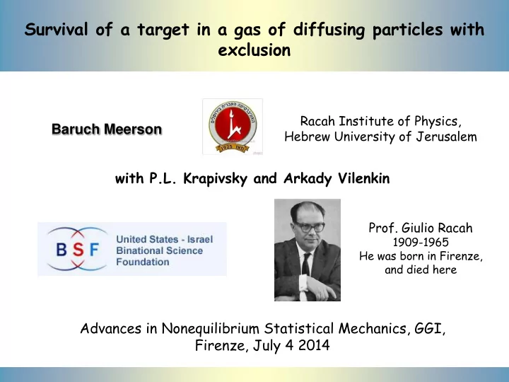
Survival of a target in a gas of diffusing particles with exclusion Racah Institute of Physics, Baruch Meerson Hebrew University of Jerusalem with P.L. Krapivsky and Arkady Vilenkin Prof. Giulio Racah 1909-1965 He was born in Firenze, and died here Advances in Nonequilibrium Statistical Mechanics, GGI, Firenze, July 4 2014

Plan  Macroscopic Fluctuation Theory of diffusive lattice gases  MFT in non-stationary settings: examples  Survival of a target against “searchers” a. Stationary fluctuations: d>2, long times b. Non-stationary fluctuations: d=1, and any d for intermediate times  Extensions and summary

Diffusive lattice gases SSEP: simple symmetric exclusion process RWs, ZRP: a = a (n i ) random walkers; zero-range process Large-scale behavior: fluctuating hydrodynamics   , x: Gaussian noise,            ξ D ( ) ( ) ( , t ) delta-correlated in x and t x t Spohn 1991, Kipnis and Landim 1999 Diffusive lattice gases are fully characterized, at large scales, by the diffusivity D (  ) and mobility  (  )

             ξ D ( ) ( ) ( , t ) x t D (  ) and  (  ) are related to the equilibrium free energy density F (  ):   2 d F ( ) 2 D ( )     2 d ( ) When noise is ignored: diffusion equation           D ( ) t

Macroscopic Fluctuation Theory (MFT) Bertini, De Sole, Gabrielli, Jona-Lasinio and Landim (2001 , …) Large parameter: number of particles in a relevant region of space. Generalizes the weak-noise WKB theory of Freidlin and Wentzel to fields Similar in spirit: Elgart and Kamenev (2004), M and Sasorov (2010) – WKB approximation to master equation for random walk on lattice and on-site reactions . Large parameter: number of particles on a single site MFT can be derived from fluctuating hydrodynamics via saddle-point expansion of a proper path integral (Tailleur, Kurchan, Lecomte 2007). This leads to a minimization problem that can be cast into a classical Hamiltonian field theory for the particle density q(x,t) and conjugate “momentum” density p(x,t):         q [ D ( q ) q ( q ) p )]     t q H / p , t 1             p H / q , 2 2 p D ( q ) p ' ( q )( p ) t t 2   H, H [ q ( , t ), p ( , t )] d x x x 1         H 2 D ( q ) q p ( q )( p ) 2

        q [ D ( q ) q ( q ) p )] t 1        2 2 p D ( q ) p ' ( q )( p ) t 2 Boundary conditions, in x and t, are determined by specific problem. Mean-field (noiseless) limit: p( x ,t)=0: downhill trajectories        q D ( q ) q t Fluctuations: p( x ,t )≠ 0: uphill trajectories, the optimal density history The probability density of a large deviation is given by the mechanical action along a proper uphill trajectory: T          P H ln S d dt p ( , t ) q ( , t ) x x x t 0 T 1      2 d dt ( q )( p ) x 2 0 If the initial condition is random, one should also find the optimal initial density profile and add to S the Boltzmann- Gibbs free energy “cost” of creating it

MFT emerged in the context of non-equilibrium steady states of lattice gases ρ - ρ + L Expected density profile solves the steady-state mean-field problem    D ( ) d / dx const         (x 0) (x L)         Density fluctuations P [ ( x )] ~ exp L F [ ( x / L )] L 1 F  large deviation functional [ ( x / L )] Reviews: Derrida 2007, Jona-Lasinio 2010, Bertini et al 2014

MFT emerged in the context of non-equilibrium steady states of lattice gases ρ - ρ + L   A ( , ) Average current    J L     P Fluctuations of current ( J ) ~ exp[ L S ( J , , )], L 1      large deviation function S ( J , , )  What is the most probable density profile for given J ? Reviews: Derrida 2007, Jona-Lasinio 2010, Bertini et al. 2014

MFT emerged in the context of non-equilibrium steady states of lattice gases ρ - ρ + L • Non-locality: long range correlations • Uphill trajectory is different from time-reversed downhill trajectory • Non-smooth parameter dependence of large deviation function/functional: “phase transitions” Reviews: Derrida 2007, Jona-Lasinio 2010, Bertini et al. 2014

Non-stationary settings are also interesting Example 1: Formation of void of size L at time T in an initially uniform gas Krapivsky, M and Sasorov 2012 n L    P d / 2 ( L , T ) ~ exp[ T S ( , n )], T 1 , L 1 d T d: dimension of space L large deviation function; Most probable density history S d ( , n ) T

Non-stationary settings are also interesting Example 2: Fluctuations of mass/energy transfer in finite time Derrida and Gerschenfeld 2009a,2009b, Sethuraman and Varadhan 2011, Krapivsky and M 2012, M and Sasorov 2013, 2014, Vilenkin, M and Sasorov 2014           M T [ ( x , T ) ( x , 0 )] dx 0    for Random Walkers     M T T , T 1 (RWs), SSEP and KMP  M     P T ( M ) ~ exp[ T S ( , , )], T 1   T T M         Large deviation function Even is nontrivial T S ( , , ) ?   T What is the most probable history of the density field conditional on M T ?

Non-stationary settings Example 3 (this talk): Target survival problem n 0 Diffusion-controlled reactions R Smoluchowski 1917 What is the probability that no particle hit the target until t=T? What is the most probable density history of the gas conditional on the non-hitting? For a given lattice gas, the answers depend on three parameters: R l  , d , n 0 DT

The T → ∞ asymptotic of the target survival probability is known for ideal gas (RWs), see references in Bray, Majumdar and Schehr, Adv. Phys. 62 , 225 (2013) Most probable density histories have not been found even for ideal gas. For non-ideal gases such as SSEP there are no previous results, except for some bounds.

MFT formulation is similar to that for the mass transfer:         q [ D ( q ) q ( q ) p )] + spherical symmetry t 1        2 2 p D ( q ) p ' ( q )( p ) t 2   Boundary condition: q ( r R , t ) 0 The process is conditional on N absorbed particles by time T:   d / 2 2     d 1 M and Redner 2014 dr r [ n q ( r , T )] N  0 ( d / 2 ) R This integral constraint calls for a Lagrangian multiplier  and leads to additional boundary condition (in time) coming from the minimization of action:     p ( r , t T ) ( r R ) The parameter  is ultimately fixed by N=0

   Deterministic, or quenched, initial condition q ( r R , t 0 ) n 0 Once q(r,t) and p(r,t) found:   T d / 2         P d 1 2 ln S(N) dt dr r ( q )( p )  r ( d / 2 ) 0 R Random, or annealed initial condition introduces two changes: • the initial condition becomes p-dependent: q ( r , 0 ) D ( q )      1 p ( r , 0 ) 2 dq ( r R ) ( 1 )  1 ( q ) 1 n 0 (Derrida and Gerschenfeld 2009) • when evaluating the probability, one should add to S the Boltzmann-Gibbs free energy “cost” of creating the optimal initial density profile q(r,0) described by Eq. (1)

Dynamic scaling of the absorption probability MFT equations are invariant under rescaling   t / T t , / DT x x  The radius of absorber becomes l R / DT   N    P d / 2 ln S ( DT ) s  l , , n  , 0 d / 2   ( DT ) We are interested in the limit N->0   1 d / 2       d 1 2 s dt dr r ( q )( p )  r ( d / 2 ) 0 l d=1: S is independent of R, so s doesn’t depend on l leading to survival probability   P 1 / 2 for all diffusive lattice gases ln ( DT ) s ( n ) 1 0 The T 1/2 scaling signals that the 1d-problem is non-stationary. An important consequence is that s 1 (n 0 ) depends on whether the initial condition is deterministic or random.

Long-time asymptotics for d>2: stationary fluctuations dq     D ( q ) ( q ) v 0 zero flux at all times dr   D ( q ) d 1      d 1 2 r v ' ( q ) v 0 , v dp / dr  d 1 r dr 2 This leads to a single nonlinear ODE for q(r):  2     D ' ' dq         2 q 0, where  r     D 2 dr   1 d d      2 d 1 q r  r   d 1 r dr dr