The FEniCS Project Anders Logg (and many others) Simula Research - PowerPoint PPT Presentation

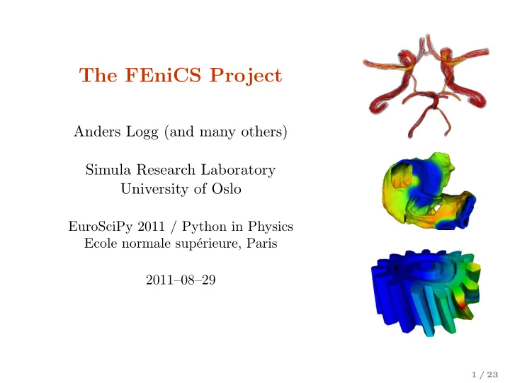
The FEniCS Project Anders Logg (and many others) Simula Research Laboratory University of Oslo EuroSciPy 2011 / Python in Physics Ecole normale sup´ erieure, Paris 2011–08–29 1 / 23

What is FEniCS? 2 / 23

FEniCS is an automated programming environment for differential equations • C++/Python library • Initiated 2003 in Chicago • 1000–2000 monthly downloads • Part of Debian and Ubuntu • Licensed under the GNU LGPL http://www.fenicsproject.org/ Collaborators Simula Research Laboratory, University of Cambridge, University of Chicago, Texas Tech University, KTH Royal Institute of Technology, . . . 3 / 23

FEniCS is automated FEM • Automated generation of basis functions • Automated evaluation of variational forms • Automated finite element assembly • Automated adaptive error control 4 / 23

What has FEniCS been used for? 5 / 23

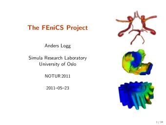
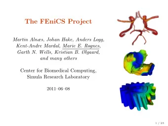
Computational hemodynamics • Low wall shear stress may trigger aneurysm growth • Solve the incompressible Navier–Stokes equations on patient-specific geometries u + ∇ u · u − ∇ · σ ( u, p ) = f ˙ ∇ · u = 0 Valen-Sendstad, Mardal, Logg, Computational hemodynamics (2011) 6 / 23

Computational hemodynamics (contd.) # Define Cauchy stress tensor def sigma(v,w): return 2.0*mu*0.5*(grad(v) + grad(v).T) - w*Identity(v.cell ().d) # Define symmetric gradient def epsilon(v): return 0.5*(grad(v) + grad(v).T) # Tentative velocity step (sigma formulation) U = 0.5*(u0 + u) F1 = rho*(1/k)*inner(v, u - u0)*dx + rho*inner(v, grad(u0)*(u0 - w))*dx \ + inner(epsilon(v), sigma(U, p0))*dx \ + inner(v, p0*n)*ds - mu*inner(grad(U).T*n, v)*ds \ - inner(v, f)*dx a1 = lhs(F1) L1 = rhs(F1) # Pressure correction a2 = inner(grad(q), k*grad(p))*dx L2 = inner(grad(q), k*grad(p0))*dx - q*div(u1)*dx # Velocity correction a3 = inner(v, u)*dx L3 = inner(v, u1)*dx + inner(v, k*grad(p0 - p1))*dx • The Navier–Stokes solver is implemented in Python/FEniCS • FEniCS allows solver to be implemented in a minimal amount of code Valen-Sendstad, Mardal, Logg, Computational hemodynamics (2011) 7 / 23

Hyperelasticity class Twist( StaticHyperelasticity ): def mesh(self): n = 8 return UnitCube(n, n, n) def dirichlet_conditions (self): clamp = Expression (("0.0", "0.0", "0.0")) twist = Expression (("0.0", "y0 + (x[1]-y0)*cos(theta) - (x[2]-z0)*sin(theta) - x[1]", "z0 + (x[1]-y0)*sin(theta) + (x[2]-z0)*cos(theta) - x[2]")) twist.y0 = 0.5 twist.z0 = 0.5 twist.theta = pi/3 return [clamp , twist] def dirichlet_boundaries (self): return ["x[0] == 0.0", "x[0] == 1.0"] def material_model (self): mu = 3.8461 lmbda = Expression("x[0]*5.8+(1-x[0])*5.7") material = StVenantKirchhoff ([mu , lmbda]) return material def __str__(self): return "A cube twisted by 60 degrees" • CBC.Solve is a collection of FEniCS-based solvers developed at CBC • CBC.Twist, CBC.Flow, CBC.Swing, CBC.Beat, . . . H. Narayanan, A computational framework for nonlinear elasticity (2011) 8 / 23

How to use FEniCS? 9 / 23

Installation Official packages for Debian and Ubuntu Drag and drop installation on Mac OS X Binary installer for Windows • Binaries for Debian, Ubuntu, Mac OS X, Windows • Automated installation from source 10 / 23

Hello World in FEniCS: problem formulation Poisson’s equation − ∆ u = f in Ω u = 0 on ∂ Ω Finite element formulation Find u ∈ V such that � � ∇ u · ∇ v d x = f v d x ∀ v ∈ V Ω Ω � �� � � �� � a ( u,v ) L ( v ) 11 / 23

Hello World in FEniCS: implementation from dolfin import * mesh = UnitSquare(32 , 32) V = FunctionSpace (mesh , "Lagrange", 1) u = TrialFunction (V) v = TestFunction(V) f = Expression("x[0]*x[1]") a = dot(grad(u), grad(v))*dx L = f*v*dx bc = DirichletBC(V, 0.0, DomainBoundary ()) u = Function(V) solve(a == L, u, bc) plot(u) 12 / 23

Hello World in FEniCS: implementation from dolfin import * mesh = UnitSquare(32 , 32) V = FunctionSpace (mesh , "Lagrange", 1) u = TrialFunction (V) v = TestFunction(V) f = Expression("x[0]*x[1]") a = dot(grad(u), grad(v))*dx L = f*v*dx bc = DirichletBC(V, 0.0, DomainBoundary ()) A = assemble(a) b = assemble(L) bc.apply(A, b) u = Function(V) solve(A, u.vector (), b) plot(u) 13 / 23

Implementation of advanced solvers in FEniCS Residuals FSISolver PrimalSolver DualSolver CBC.Flow CBC.Twist MeshSolver K. Selim, An adaptive finite element solver for fluid–structure interaction problems (2011) 14 / 23

Implementation of advanced solvers in FEniCS # Tentative velocity step (sigma formulation) # Time -stepping loop U = 0.5*(u0 + u) while True: F1 = rho*(1/k)*inner(v, u - u0)*dx + rho*inner(v, grad(u0)*(u0 - w))*dx \ # Fixed point iteration on FSI problem + inner(epsilon(v), sigma(U, p0))*dx \ for iter in range(maxiter): + inner(v, p0*n)*ds - mu*inner(grad(U).T*n, v)*ds \ - inner(v, f)*dx # Solve fluid subproblem a1 = lhs(F1) F.step(dt) L1 = rhs(F1) # Transfer fluid stresses to structure class StVenantKirchhoff (MaterialModel): Sigma_F = F. compute_fluid_stress (u_F0 , u_F1 , p_F0 , p_F1 , def model_info(self): U_M0 , U_M1) self.num_parameters = 2 S. update_fluid_stress (Sigma_F) self. kinematic_measure = \ " GreenLagrangeStrain " # Solve structure subproblem U_S1 , P_S1 = S.step(dt) def strain_energy(self , parameters): E = self.E # Transfer structure displacement to fluidmesh [mu , lmbda] = parameters M. update_structure_displacement (U_S1) return lmbda/2*(tr(E)**2) + mu*tr(E*E) # Solve mesh equation M.step(dt) class GentThomas(MaterialModel): # Transfer mesh displacement to fluid def model_info(self): F. update_mesh_displacement (U_M1 , dt) self.num_parameters = 2 self. kinematic_measure = \ " CauchyGreenInvariants " # Fluid residual contributions R_F0 = w*inner(EZ_F - Z_F , Dt_U_F - div(Sigma_F ))*dx_F def strain_energy(self , parameters): R_F1 = avg(w)*inner(EZ_F(’+’) - Z_F(’+’), I1 = self.I1 jump(Sigma_F , N_F))*dS_F I2 = self.I2 R_F2 = w*inner(EZ_F - Z_F , dot(Sigma_F , N_F))*ds R_F3 = w*inner(EY_F - Y_F , [C1 , C2] = parameters div(J(U_M)*dot(inv(F(U_M)), U_F )))*dx_F return C1*(I1 - 3) + C2*ln(I2/3) 15 / 23

Basic API • Mesh , MeshEntity , Vertex , Edge , Face , Facet , Cell • FiniteElement , FunctionSpace • TrialFunction , TestFunction , Function • grad() , curl() , div() , . . . • Matrix , Vector , KrylovSolver • assemble() , solve() , plot() • Python interface generated semi-automatically by SWIG • C++ and Python interfaces almost identical 16 / 23

FEniCS under the hood 17 / 23

Automated scientific computing Output Input • u h ≈ u • A ( u ) = f • � u − u h � ≤ ǫ • ǫ > 0 18 / 23

Automatic code generation Input Equation (variational problem) Output Efficient application-specific code 19 / 23

Code generation system mesh = UnitSquare(32, 32) V = FunctionSpace(mesh, "Lagrange", 1) u = TrialFunction(V) v = TestFunction(V) f = Expression("x[0]*x[1]") a = dot(grad(u), grad(v))*dx L = f*v*dx bc = DirichletBC(V, 0.0, DomainBoundary()) A = assemble(a) b = assemble(L) bc.apply(A, b) u = Function(V) solve(A, u.vector(), b) 20 / 23

Code generation system mesh = UnitSquare(32, 32) V = FunctionSpace(mesh, "Lagrange", 1) u = TrialFunction(V) v = TestFunction(V) f = Expression("x[0]*x[1]") a = dot(grad(u), grad(v))*dx L = f*v*dx bc = DirichletBC(V, 0.0, DomainBoundary()) A = assemble(a) b = assemble(L) bc.apply(A, b) u = Function(V) solve(A, u.vector(), b) (Python, C++–SWIG–Python, Python–JIT–C++–GCC–SWIG–Python) 20 / 23

FEniCS software components Applications FEniCS Apps Application Application Interfaces Puffin DOLFIN Core components SyFi Viper UFL UFC FFC FIAT Instant FErari External libraries PETSc uBLAS UMFPACK NumPy SCOTCH VTK Trilinos GMP ParMETIS CGAL MPI SLEPc 21 / 23

Closing remarks 22 / 23

Current and future activities • Parallelization (2009) • Automated error control (2010) • Debian/Ubuntu (2010) • Documentation (2010) • 1.0-beta (Aug 2011) • Release of 1.0 (2011) • Book (2011) • New web page (2011) • FEniCS’11 at Texas Tech http://www.fenicsproject.org/ 23 / 23