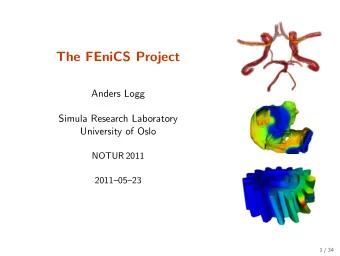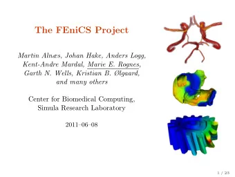
The FEniCS Project Presented by Anders Logg Simula Research - PowerPoint PPT Presentation

The FEniCS Project Presented by Anders Logg ∗ Simula Research Laboratory, Oslo University of Chicago 2012–10–09 ∗ Credits: http://fenicsproject.org/about/team.html 1 / 40

What is FEniCS? 2 / 40

FEniCS is an automated programming environment for differential equations • C++/Python library • Initiated 2003 in Chicago • 1000–2000 monthly downloads • Part of Debian and Ubuntu • Licensed under the GNU LGPL http://fenicsproject.org/ Collaborators Simula Research Laboratory, University of Cambridge, University of Chicago, Texas Tech University, University of Texas at Austin, KTH Royal Institute of Technology, . . . 3 / 40

FEniCS is automated FEM • Automated generation of basis functions • Automated evaluation of variational forms • Automated finite element assembly • Automated adaptive error control 4 / 40

FEniCS is automated scientific computing Input • A ( u ) = f • ǫ > 0 Output • Approximate solution: u h ≈ u • Guaranteed accuracy: � u − u h � ≤ ǫ 5 / 40

How to use FEniCS? 6 / 40

Installation Official packages for Debian and Ubuntu Drag and drop installation on Mac OS X Binary installer for Windows Automated installation from source 7 / 40

Hello World in FEniCS: problem formulation Poisson’s equation − ∆ u = f in Ω u = 0 on ∂ Ω Finite element formulation Find u ∈ V such that � � ∇ u · ∇ v d x = f v d x ∀ v ∈ V Ω Ω � �� � � �� � a ( u,v ) L ( v ) 8 / 40

Hello World in FEniCS: implementation from dolfin import * mesh = UnitSquare(32 , 32) V = FunctionSpace (mesh , "Lagrange", 1) u = TrialFunction (V) v = TestFunction(V) f = Expression("x[0]*x[1]") a = dot(grad(u), grad(v))*dx L = f*v*dx bc = DirichletBC(V, 0.0, DomainBoundary ()) u = Function(V) solve(a == L, u, bc) plot(u) 9 / 40

Linear elasticity Differential equation Differential equation: −∇ · σ ( u ) = f where σ ( v ) = 2 µǫ ( v ) + λ tr ǫ ( v ) I ǫ ( v ) = 1 2( ∇ v + ( ∇ v ) ⊤ ) • Displacement u = u ( x ) • Stress σ = σ ( x ) 10 / 40

Linear elasticity Variational formulation Find u ∈ V such that ∀ v ∈ ˆ a ( u, v ) = L ( v ) V where a ( u, v ) = � σ ( u ) , ǫ ( v ) � L ( v ) = � f, v � 10 / 40

Linear elasticity Implementation element = VectorElement("Lagrange", "tetrahedron", 1) v = TestFunction(element) u = TrialFunction(element) f = Function(element) def epsilon(v): return 0.5*(grad(v) + grad(v).T) def sigma(v): return 2.0*mu*epsilon(v) + lmbda*tr(epsilon(v))*I a = inner(sigma(u), epsilon(v))*dx L = dot(f, v)*dx 10 / 40

Poisson’s equation with DG elements Differential equation Differential equation: − ∆ u = f • u ∈ L 2 • u discontinuous across element boundaries 11 / 40

Poisson’s equation with DG elements Variational formulation (interior penalty method) Find u ∈ V such that a ( u, v ) = L ( v ) ∀ v ∈ V where � a ( u, v ) = ∇ u · ∇ v d x Ω � � + −�∇ u � · � v � n − � u � n · �∇ v � + ( α/h ) � u � n · � v � n d S S S � + −∇ u · � v � n − � u � n · ∇ v + ( γ/h ) uv d s ∂ Ω � � L ( v ) = fv d x + gv d s Ω ∂ Ω 11 / 40

Poisson’s equation with DG elements Implementation V = FunctionSpace(mesh, "DG", 1) u = TrialFunction(V) v = TestFunction(V) f = Expression(...) g = Expression(...) n = FacetNormal(mesh) h = CellSize(mesh) a = dot(grad(u), grad(v))*dx - dot(avg(grad(u)), jump(v, n))*dS - dot(jump(u, n), avg(grad(v)))*dS + alpha/avg(h)*dot(jump(u, n), jump(v, n))*dS - dot(grad(u), jump(v, n))*ds - dot(jump(u, n), grad(v))*ds + gamma/h*u*v*ds Oelgaard, Logg, Wells, Automated Code Generation for Discontinuous Galerkin Methods (2008) 11 / 40

Simple prototyping and development in Python # Tentative velocity step (sigma formulation) # Time -stepping loop U = 0.5*(u0 + u) while True: F1 = rho*(1/k)*inner(v, u - u0)*dx + rho*inner(v, grad(u0)*(u0 - w))*dx \ # Fixed point iteration on FSI problem + inner(epsilon(v), sigma(U, p0))*dx \ for iter in range(maxiter): + inner(v, p0*n)*ds - mu*inner(grad(U).T*n, v)*ds \ - inner(v, f)*dx # Solve fluid subproblem a1 = lhs(F1) F.step(dt) L1 = rhs(F1) # Transfer fluid stresses to structure class StVenantKirchhoff (MaterialModel): Sigma_F = F. compute_fluid_stress (u_F0 , u_F1 , p_F0 , p_F1 , def model_info(self): U_M0 , U_M1) self.num_parameters = 2 S. update_fluid_stress (Sigma_F) self. kinematic_measure = \ " GreenLagrangeStrain " # Solve structure subproblem U_S1 , P_S1 = S.step(dt) def strain_energy(self , parameters): E = self.E # Transfer structure displacement to fluidmesh [mu , lmbda] = parameters M. update_structure_displacement (U_S1) return lmbda/2*(tr(E)**2) + mu*tr(E*E) # Solve mesh equation M.step(dt) class GentThomas(MaterialModel): # Transfer mesh displacement to fluid def model_info(self): F. update_mesh_displacement (U_M1 , dt) self.num_parameters = 2 self. kinematic_measure = \ " CauchyGreenInvariants " # Fluid residual contributions R_F0 = w*inner(EZ_F - Z_F , Dt_U_F - div(Sigma_F ))*dx_F def strain_energy(self , parameters): R_F1 = avg(w)*inner(EZ_F(’+’) - Z_F(’+’), I1 = self.I1 jump(Sigma_F , N_F))*dS_F I2 = self.I2 R_F2 = w*inner(EZ_F - Z_F , dot(Sigma_F , N_F))*ds R_F3 = w*inner(EY_F - Y_F , [C1 , C2] = parameters div(J(U_M)*dot(inv(F(U_M)), U_F )))*dx_F return C1*(I1 - 3) + C2*ln(I2/3) 12 / 40

Simple development of specialized applications # Define Cauchy stress tensor def sigma(v,w): return 2.0*mu*0.5*(grad(v) + grad(v).T) - w*Identity(v.cell ().d) # Define symmetric gradient def epsilon(v): return 0.5*(grad(v) + grad(v).T) # Tentative velocity step (sigma formulation) U = 0.5*(u0 + u) F1 = rho*(1/k)*inner(v, u - u0)*dx + rho*inner(v, grad(u0)*(u0 - w))*dx \ + inner(epsilon(v), sigma(U, p0))*dx \ + inner(v, p0*n)*ds - mu*inner(grad(U).T*n, v)*ds \ - inner(v, f)*dx a1 = lhs(F1) L1 = rhs(F1) # Pressure correction a2 = inner(grad(q), k*grad(p))*dx L2 = inner(grad(q), k*grad(p0))*dx - q*div(u1)*dx # Velocity correction a3 = inner(v, u)*dx L3 = inner(v, u1)*dx + inner(v, k*grad(p0 - p1))*dx • The Navier–Stokes solver is implemented in Python/FEniCS • FEniCS allows solvers to be implemented in a minimal amount of code • Simple integration with application specific code and data management Valen-Sendstad, Mardal, Logg, Computational hemodynamics (2011) 13 / 40

FEniCS under the hood 14 / 40

Automatic code generation Input Equation (variational problem) Output Efficient application-specific code 15 / 40

Code generation framework • UFL - Unified Form Language • UFC - Unified Form-assembly Code • Form compilers: FFC, SyFi a ( u, v ) = �∇ u, ∇ v � 16 / 40

Form compiler interfaces Command-line >> ffc poisson.ufl Just-in-time V = FunctionSpace(mesh, "CG", 3) u = TrialFunction(V) v = TestFunction(V) A = assemble(dot(grad(u), grad(v))*dx) 17 / 40

Code generation system mesh = UnitSquare(32, 32) V = FunctionSpace(mesh, "Lagrange", 1) u = TrialFunction(V) v = TestFunction(V) f = Expression("x[0]*x[1]") a = dot(grad(u), grad(v))*dx L = f*v*dx bc = DirichletBC(V, 0.0, DomainBoundary()) A = assemble(a) b = assemble(L) bc.apply(A, b) u = Function(V) solve(A, u.vector(), b) 18 / 40

Code generation system mesh = UnitSquare(32, 32) V = FunctionSpace(mesh, "Lagrange", 1) u = TrialFunction(V) v = TestFunction(V) f = Expression("x[0]*x[1]") a = dot(grad(u), grad(v))*dx L = f*v*dx bc = DirichletBC(V, 0.0, DomainBoundary()) A = assemble(a) b = assemble(L) bc.apply(A, b) u = Function(V) solve(A, u.vector(), b) (Python, C++–SWIG–Python, Python–JIT–C++–GCC–SWIG–Python) 18 / 40

Just-In-Time (JIT) compilation 19 / 40

Geometry and meshing 20 / 40

Geometry and meshing Built-in meshing mesh = UnitSquare(64 , 64) mesh = UnitCube(64 , 64 , 64) External mesh generators mesh = Mesh("mesh.xml") dolfin-convert mesh.inp mesh.xml Conversion from Gmsh, Medit, Tetgen, Diffpack, Abaqus, ExodusII, Star-CD Extensions / work in progress • Constructive solid geometry (CSG) • Meshing from biomedical image data using VMTK 21 / 40

Constructive solid geometry (CSG) Boolean operators A ∪ B A + B A ∩ B A * B A \ B A - B Implementation • Modeled after NETGEN • Implemented using CGAL Example r = Rectangle(-1, -1, 1, 1) c = Circle(0, 0, 1) g = c - r mesh = Mesh(g) 22 / 40

Meshing from biomedical images • Biomedical image data (DICOM) • VMTK generates high quality FEniCS meshes • Adaptive a priori graded meshes • Simple specification of boundary markers • Resolution of boundary layers Antiga, Mardal, Valen-Sendstad, Tangui Morvan 23 / 40

Meshing from biomedical images • Biomedical image data (DICOM) • VMTK generates high quality FEniCS meshes • Adaptive a priori graded meshes • Simple specification of boundary markers • Resolution of boundary layers Antiga, Mardal, Valen-Sendstad, Tangui Morvan 23 / 40

Meshing from biomedical images • Biomedical image data (DICOM) • VMTK generates high quality FEniCS meshes • Adaptive a priori graded meshes • Simple specification of boundary markers • Resolution of boundary layers Antiga, Mardal, Valen-Sendstad, Tangui Morvan 23 / 40