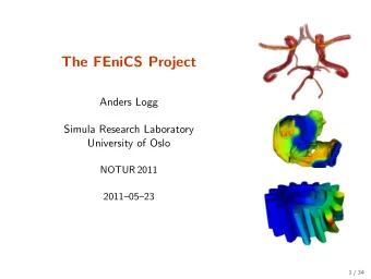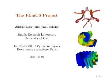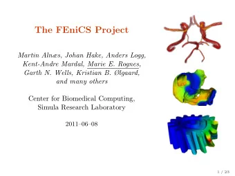
The FEniCS Project Anders Logg Simula Research Laboratory / - PowerPoint PPT Presentation

The FEniCS Project Anders Logg Simula Research Laboratory / University of Oslo Det Norske Veritas 2011–05–11

The FEniCS Project Free Software for Automated Scientific Computing • C++/Python library • Initiated 2003 in Chicago • 1000–2000 monthly downloads • Part of Debian/Ubuntu GNU/Linux • Licensed under the GNU LGPL http://www.fenicsproject.org/ Collaborators University of Chicago, Argonne National Laboratory, Delft University of Technology, Royal Institute of Technology KTH, Simula Research Laboratory, Texas Tech University, University of Cambridge , . . .

Key Features • Simple and intuitive object-oriented API, C++ or Python • Automatic and efficient evaluation of variational forms • Automatic and efficient assembly of linear systems • Distributed (clusters) and shared memory (multicore) parallelism • General families of finite elements, including arbitrary order continuous and discontinuous Lagrange elements, BDM, RT, Nedelec, . . . • Arbitrary mixed elements • High-performance parallel linear algebra • General meshes, adaptive mesh refinement • mcG( q )/mdG( q ) and cG( q )/dG( q ) ODE solvers • Support for a range of input/output formats • Built-in plotting

The State of FEniCS • Parallelization (2009) • Automated error control (2010) • Debian/Ubuntu (2010) • Documentation (2010) • Latest release: 0.9.10 (Feb 2011) • Release of 1.0 (2011) • Book (2011) • New web page (2011)

Outline • Automated Scientific Computing • Interface and Design • Examples and Applications

Automated Scientific Computing

Automated Scientific Computing Input • A ( u ) = f • ǫ > 0 Output � u − u h � ≤ ǫ

Blueprint

Key Steps Key steps (i) Automated discretization (2006) (ii) Automated error control (2010) (iii) Automated discrete solution . . . Key techniques • Adaptive finite element methods • Automatic code generation

Automatic Code Generation Input Equation (variational problem) Output Efficient application-specific code

Speedup • CPU time for computing the “element stiffness matrix” • Straight-line C++ code generated by the FEniCS Form Compiler (FFC) • Speedup vs a standard quadrature-based C++ code with loops over quadrature points • Recently, optimized quadrature code has been shown to be competitive [Oelgaard/Wells, TOMS 2009] Form q = 1 q = 2 q = 3 q = 4 q = 5 q = 6 q = 7 q = 8 Mass 2D 12 31 50 78 108 147 183 232 Mass 3D 21 81 189 355 616 881 1442 1475 Poisson 2D 8 29 56 86 129 144 189 236 Poisson 3D 9 56 143 259 427 341 285 356 Navier–Stokes 2D 32 33 53 37 — — — — Navier–Stokes 3D 77 100 61 42 — — — — Elasticity 2D 10 43 67 97 — — — — Elasticity 3D 14 87 103 134 — — — —

Interface and Design

A Simple Example − ∆ u + u = f in Ω ∂ n u = 0 on ∂ Ω Canonical variational problem Find u ∈ V such that ∀ v ∈ ˆ a ( u, v ) = L ( v ) V where a ( u, v ) = �∇ u, ∇ v � + � u, v � L ( v ) = � f, v � Here: V = ˆ V = H 1 (Ω ), f ( x, y ) = sin x sin y , Ω = (0 , 1) × (0 , 1)

Programming in FEniCS Complete code (Python) from dolfin import * # Define variational problem mesh = UnitSquare(32, 32) V = FunctionSpace(mesh, "CG", 1) u = TrialFunction(V) v = TestFunction(V) f = Expression("sin(x[0])*sin(x[1])") a = (grad(u), grad(v)) + (u, v) L = (f, v) # Compute and plot solution problem = VariationalProblem(a, L) u = problem.solve() plot(u)

Design Considerations • Simple and minimal interfaces • Efficient backends • Object-oriented API (but not too much) • Code genereration (but not too much) • Application-driven development • Technology-driven development

Basic API • Mesh , MeshEntity , Vertex , Edge , Face , Facet , Cell • FiniteElement , FunctionSpace • TrialFunction , TestFunction , Function • grad() , curl() , div() , . . . • Matrix , Vector , KrylovSolver • assemble() , solve() , plot() • Python interface generated semi-automatically by SWIG • C++ and Python interfaces almost identical

DOLFIN Class Diagram

Assembler Interfaces

Linear Algebra in DOLFIN • Generic linear algebra interface to • PETSc • Trilinos/Epetra • uBLAS • MTL4 • Eigenvalue problems solved by SLEPc for PETSc matrix types • Matrix-free solvers (“virtual matrices”) Linear algebra backends >>> from dolfin import * >>> parameters["linear_algebra_backend"] = "PETSc" >>> A = Matrix() >>> parameters["linear_algebra_backend"] = "Epetra" >>> B = Matrix()

Code Generation System from dolfin import * mesh = UnitSquare(32, 32) V = FunctionSpace(mesh, "CG", 1) u = TrialFunction(V) v = TestFunction(V) f = Expression("sin(x[0])*sin(x[1])") a = (grad(u), grad(v)) + (u, v) L = (f, v) A = assemble(a, mesh) b = assemble(L, mesh) u = Function(V) solve(A, u.vector(), b) plot(u) (Python, C++ – SWIG – Python, Python – JIT – C++ – GCC – SWIG – Python)

Code Generation System from dolfin import * mesh = UnitSquare(32, 32) V = FunctionSpace(mesh, "CG", 1) u = TrialFunction(V) v = TestFunction(V) f = Expression("sin(x[0])*sin(x[1])") a = (grad(u), grad(v)) + (u, v) L = (f, v) A = assemble(a, mesh) b = assemble(L, mesh) u = Function(V) solve(A, u.vector(), b) plot(u) (Python, C++ – SWIG – Python, Python – JIT – C++ – GCC – SWIG – Python)

FEniCS Software Components Applications FEniCS Apps Application Application Interfaces DOLFIN Puffin Core components SyFi Viper UFL UFC FFC FIAT Instant FErari External libraries PETSc uBLAS UMFPACK NumPy SCOTCH VTK Trilinos GMP ParMETIS CGAL MPI SLEPc

Installation Official packages for Debian and Ubuntu Drag and drop installation on Mac OS X (requires XCode) Binary installer for Windows (based on MinGW) • Automated building from source for a multitude of platforms (using Dorsal) • VirtualBox / VMWare + Ubuntu!

Nightly Testing

Examples and Applications

Poisson’s Equation Differential equation − ∆ u = f • Heat transfer • Electrostatics • Magnetostatics • Fluid flow • etc.

Poisson’s Equation Variational formulation Find u ∈ V such that a ( u, v ) = L ( v ) ∀ v ∈ V where a ( u, v ) = �∇ u, ∇ v � L ( v ) = � f, v �

Poisson’s Equation Implementation V = FunctionSpace(mesh, "CG", 1) u = TrialFunction(V) v = TestFunction(V) f = Expression(...) a = (grad(u), grad(v)) L = (f, v)

Mixed Poisson with H (div) Elements Differential equation σ + ∇ u = 0 ∇ · σ = f • u ∈ L 2 • σ ∈ H (div)

Mixed Poisson with H (div) Elements Variational formulation Find ( σ, u ) ∈ V such that a (( σ, u ) , ( τ, v )) = L (( τ, v )) ∀ ( τ, v ) ∈ V where a (( σ, u ) , ( τ, v )) = � σ, τ � − � u, ∇ · τ � + �∇ · σ, v � L (( τ, v )) = � f, v �

Mixed Poisson with H (div) Elements Implementation BDM1 = FunctionSpace(mesh, "BDM", 1) DG0 = FunctionSpace(mesh, "DG", 0) V = BDM1 * DG0 (sigma, u) = TrialFunctions(V) (tau, v) = TestFunctions(V) f = Expression(...) a = (sigma, tau) + (u, -div(tau)) + (div(sigma), v) L = (f, v) Rognes, Kirby, Logg, Efficient Assembly of H (div) and H (curl) Conforming Finite Elements (2009)

Poisson’s Equation with DG Elements Differential equation Differential equation: − ∆ u = f • u ∈ L 2 • u discontinuous across element boundaries

Poisson’s Equation with DG Elements Variational formulation (interior penalty method) Find u ∈ V such that a ( u, v ) = L ( v ) ∀ v ∈ V where � a ( u, v ) = ∇ u · ∇ v d x Ω � � + −�∇ u � · � v � n − � u � n · �∇ v � + ( α/h ) � u � n · � v � n d S S S � + −∇ u · � v � n − � u � n · ∇ v + ( γ/h ) uv d s ∂ Ω � � L ( v ) = fv d x + gv d s ∂ Ω Ω

Poisson’s Equation with DG Elements Implementation V = FunctionSpace(mesh, "DG", 1) u = TrialFunction(V) v = TestFunction(V) f = Expression(...) g = Expression(...) n = FacetNormal(mesh) h = MeshSize(mesh) a = dot(grad(u), grad(v))*dx - dot(avg(grad(u)), jump(v, n))*dS - dot(jump(u, n), avg(grad(v)))*dS + alpha/avg(h)*dot(jump(u, n), jump(v, n))*dS - dot(grad(u), jump(v, n))*ds - dot(jump(u, n), grad(v))*ds + gamma/h*u*v*ds Oelgaard, Logg, Wells, Automated Code Generation for Discontinuous Galerkin Methods (2008)

Computational Hemodynamics Valen-Sendstad, Mardal, Logg, Simulating the Hemodynamics of the Circle of Willis (2010)

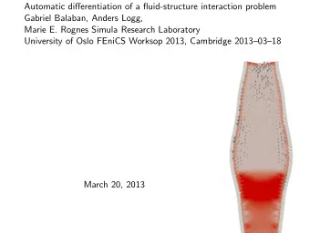
Fluid–Structure Interaction • Fluid governed by the incompressible Navier–Stokes equations • Structure governed by the nonlinear St. Venant–Kirchhoff model • Mesh and time steps determined adaptively to control the error in a given goal functional to within a given tolerance Selim, Logg, Narayanan, Larson, An Adaptive Finite Element Method for FSI (2011)

Adaptive Error Control for FSI Selim, Logg, Narayanan, Larson, An Adaptive Finite Element Method for FSI (2011)