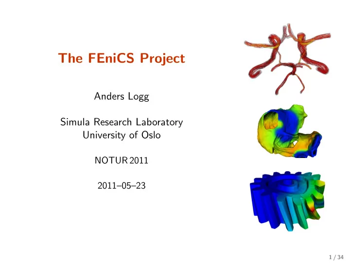
The FEniCS Project Anders Logg Simula Research Laboratory - PowerPoint PPT Presentation

The FEniCS Project Anders Logg Simula Research Laboratory University of Oslo NOTUR 2011 2011–05–23 1 / 34

What is FEniCS? 2 / 34

FEniCS is an automated programming environment for differential equations • C++/Python library • Initiated 2003 in Chicago • 1000–2000 monthly downloads • Part of Debian/Ubuntu GNU/Linux • Licensed under the GNU LGPL http://www.fenicsproject.org/ Collaborators University of Chicago, Argonne National Laboratory, Delft University of Technology, Royal Institute of Technology KTH, Simula Research Laboratory, Texas Tech University, University of Cambridge , . . . 3 / 34

FEniCS is new technology combining generality, efficiency, simplicity and reliability Generality Efficiency Code Generation • Generality through abstraction • Efficiency through code generation , adaptivity , parallelism • Simplicity through high level scripting • Reliability through adaptive error control 4 / 34

FEniCS is automated FEM • Automated generation of basis functions • Automated evaluation of variational forms • Automated finite element assembly • Automated adaptive error control 5 / 34

What has FEniCS been used for? 6 / 34

Computational hemodynamics • Low wall shear stress may trigger aneurysm growth • Solve the incompressible Navier–Stokes equations on patient-specific geometries u + ∇ u · u − ∇ · σ ( u , p ) = f ˙ ∇ · u = 0 Valen-Sendstad, Mardal, Logg, Computational hemodynamics (2011) 7 / 34

Computational hemodynamics (contd.) # Define Cauchy stress tensor def sigma(v,w): return 2.0*mu*0.5*(grad(v) + grad(v).T) - w*Identity(v.cell ().d) # Define symmetric gradient def epsilon(v): return 0.5*(grad(v) + grad(v).T) # Tentative velocity step (sigma formulation) U = 0.5*(u0 + u) F1 = rho*(1/k)*inner(v, u - u0)*dx + rho*inner(v, grad(u0)*(u0 - w))*dx \ + inner(epsilon(v), sigma(U, p0))*dx \ + inner(v, p0*n)*ds - mu*inner(grad(U).T*n, v)*ds \ - inner(v, f)*dx a1 = lhs(F1) L1 = rhs(F1) # Pressure correction a2 = inner(grad(q), k*grad(p))*dx L2 = inner(grad(q), k*grad(p0))*dx - q*div(u1)*dx # Velocity correction a3 = inner(v, u)*dx L3 = inner(v, u1)*dx + inner(v, k*grad(p0 - p1))*dx • The Navier–Stokes solver is implemented in Python/FEniCS • FEniCS allows the solver to be implemented in a minimal amount of code Valen-Sendstad, Mardal, Logg, Computational hemodynamics (2011) 8 / 34

Hyperelasticity class Twist( StaticHyperelasticity ): def mesh(self): n = 8 return UnitCube(n, n, n) def dirichlet_conditions (self): clamp = Expression (("0.0", "0.0", "0.0")) twist = Expression (("0.0", "y0 + (x[1]-y0)*cos(theta) - (x[2]-z0)*sin(theta) - x[1]", "z0 + (x[1]-y0)*sin(theta) + (x[2]-z0)*cos(theta) - x[2]")) twist.y0 = 0.5 twist.z0 = 0.5 twist.theta = pi/3 return [clamp , twist] def dirichlet_boundaries (self): return ["x[0] == 0.0", "x[0] == 1.0"] def material_model (self): mu = 3.8461 lmbda = Expression("x[0]*5.8+(1-x[0])*5.7") material = StVenantKirchhoff ([mu , lmbda]) return material def __str__(self): return "A cube twisted by 60 degrees" • CBC.Solve is a collection of FEniCS-based solvers developed at the CBC • CBC.Twist, CBC.Flow, CBC.Swing, CBC.Beat, . . . H. Narayanan, A computational framework for nonlinear elasticity (2011) 9 / 34

Fluid–structure interaction • The FSI problem is a computationally very expensive coupled multiphysics problem • The FSI problem has many important applications in engineering and biomedicine Images courtesy of the Internet 10 / 34

Fluid–structure interaction (contd.) • Fluid governed by the incompressible Navier–Stokes equations • Structure modeled by the St. Venant–Kirchhoff model • Adaptive refinement in space and time Selim, Logg, Narayanan, Larson, An Adaptive Finite Element Method for FSI (2011) 11 / 34

Computational geodynamics − div σ ′ − ∇ p = ( Rb φ − Ra T ) e div u = 0 ∂ T ∂ t + u · ∇ T = ∆ T ∂φ ∂ t + u · ∇ φ = k c ∆ φ σ ′ = 2 η ˙ ε ( u ) ε ( u ) = 1 � ∇ u + ∇ u T � ˙ 2 η = η 0 exp ( − bT / ∆ T + c ( h − x 2 ) / h ) Image courtesy of the Internet 12 / 34

Computational geodynamics (contd.) • The mantle convection simulator is implemented in Python/FEniCS • Images show a sequence of snapshots of the temperature distribution Vynnytska, Clark, Rognes, Dynamic simulations of convection in the Earth’s mantle (2011) 13 / 34

How to use FEniCS? 14 / 34

Installation Official packages for Debian and Ubuntu Drag and drop installation on Mac OS X Binary installer for Windows • Automated building from source for a multitude of platforms • VirtualBox / VMWare + Ubuntu! 15 / 34

Hello World in FEniCS: problem formulation Poisson’s equation − ∆ u = f in Ω u = 0 on ∂ Ω Finite element formulation Find u ∈ V such that � � ∀ v ∈ ˆ ∇ u · ∇ v d x = f v d x V Ω Ω 16 / 34

Hello World in FEniCS: problem formulation Poisson’s equation − ∆ u = f in Ω u = 0 on ∂ Ω Variational formulation Find u ∈ V such that � � ∀ v ∈ ˆ ∇ u · ∇ v d x = f v d x V Ω Ω � �� � � �� � a ( u , v ) L ( v ) 16 / 34

Hello World in FEniCS: implementation from dolfin import * mesh = UnitSquare(32, 32) V = FunctionSpace(mesh, "Lagrange", 1) u = TrialFunction(V) v = TestFunction(V) f = Expression("x[0]*x[1]") a = dot(grad(u), grad(v))*dx L = f*v*dx bc = DirichletBC(V, 0.0, DomainBoundary()) problem = VariationalProblem(a, L, bc) u = problem.solve() plot(u) 17 / 34

Implementation of advanced solvers in FEniCS FSISolver Residuals PrimalSolver DualSolver CBC.Flow CBC.Twist MeshSolver K. Selim, An adaptive finite element solver for fluid–structure interaction problems (2011) 18 / 34

Implementation of advanced solvers in FEniCS # Tentative velocity step (sigma formulation) # Time -stepping loop U = 0.5*(u0 + u) while True: F1 = rho*(1/k)*inner(v, u - u0)*dx + rho*inner(v, grad(u0)*(u0 - w))*dx \ # Fixed point iteration on FSI problem + inner(epsilon(v), sigma(U, p0))*dx \ for iter in range(maxiter): + inner(v, p0*n)*ds - mu*inner(grad(U).T*n, v)*ds \ - inner(v, f)*dx # Solve fluid subproblem a1 = lhs(F1) F.step(dt) L1 = rhs(F1) # Transfer fluid stresses to structure class StVenantKirchhoff (MaterialModel): Sigma_F = F. compute_fluid_stress (u_F0 , u_F1 , p_F0 , p_F1 , def model_info(self): U_M0 , U_M1) self.num_parameters = 2 S. update_fluid_stress (Sigma_F) self. kinematic_measure = \ " GreenLagrangeStrain " # Solve structure subproblem U_S1 , P_S1 = S.step(dt) def strain_energy(self , parameters): E = self.E # Transfer structure displacement to fluidmesh [mu , lmbda] = parameters M. update_structure_displacement (U_S1) return lmbda/2*(tr(E)**2) + mu*tr(E*E) # Solve mesh equation M.step(dt) class GentThomas(MaterialModel): # Transfer mesh displacement to fluid def model_info(self): F. update_mesh_displacement (U_M1 , dt) self.num_parameters = 2 self. kinematic_measure = \ " CauchyGreenInvariants " # Fluid residual contributions R_F0 = w*inner(EZ_F - Z_F , Dt_U_F - div(Sigma_F ))*dx_F def strain_energy(self , parameters): R_F1 = avg(w)*inner(EZ_F(’+’) - Z_F(’+’), I1 = self.I1 jump(Sigma_F , N_F))*dS_F I2 = self.I2 R_F2 = w*inner(EZ_F - Z_F , dot(Sigma_F , N_F))*ds R_F3 = w*inner(EY_F - Y_F , [C1 , C2] = parameters div(J(U_M)*dot(inv(F(U_M)), U_F )))*dx_F return C1*(I1 - 3) + C2*ln(I2/3) 19 / 34

Key features • Simple and intuitive object-oriented API, C++ or Python • Automatic and efficient evaluation of variational forms • Automatic and efficient assembly of linear systems • Distributed (clusters) and shared memory (multicore) parallelism • General families of finite elements, including arbitrary order continuous and discontinuous Lagrange elements, BDM, RT, N´ ed´ elec, . . . • Arbitrary mixed elements • High-performance parallel linear algebra • General meshes, adaptive mesh refinement • mcG( q )/mdG( q ) and cG( q )/dG( q ) ODE solvers • Support for a range of input/output formats • Built-in plotting 20 / 34

Basic API • Mesh , MeshEntity , Vertex , Edge , Face , Facet , Cell • FiniteElement , FunctionSpace • TrialFunction , TestFunction , Function • grad() , curl() , div() , . . . • Matrix , Vector , KrylovSolver • assemble() , solve() , plot() • Python interface generated semi-automatically by SWIG • C++ and Python interfaces almost identical 21 / 34

DOLFIN class diagram 22 / 34

FEniCS under the hood 23 / 34

Automated Scientific Computing Input • A ( u ) = f • ǫ > 0 Output � u − u h � ≤ ǫ 24 / 34

Automated Scientific Computing: a blueprint 25 / 34

Automatic code generation Input Equation (variational problem) Output Efficient application-specific code 26 / 34

Assembler interfaces 27 / 34