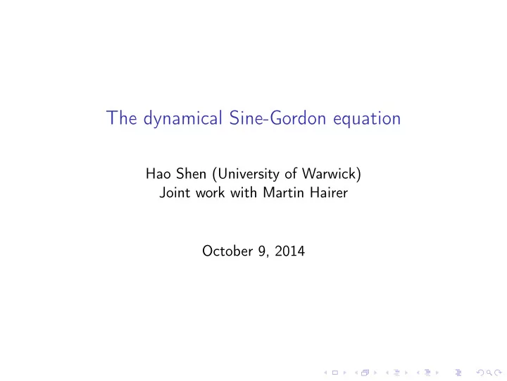
The dynamical Sine-Gordon equation Hao Shen (University of Warwick) - PowerPoint PPT Presentation

The dynamical Sine-Gordon equation Hao Shen (University of Warwick) Joint work with Martin Hairer October 9, 2014

Dynamical Sine-Gordon Equation Space dimension d = 2. Equation depends on parameter � > 0. @ t u = 1 2 ∆ u + ⇣ sin ( � u ) + ⇠ ⇠ is space-time white noise.

Some parabolic stochastic PDEs I Stochastic heat equation ( ⇠ space-time white noise) (Walsh 1980s) @ t u = ∆ u + ⇠ I KPZ (Bertini-Giacomin 1997, Hairer 2011, Hairer-Quastel) @ t h = ∆ h + ( r h ) 2 + ⇠ I Dynamical Φ 4 (Da Prato-Debussche 2003, Hairer 2013, Mourrat-Weber 2014, Hairer-Xu) @ t � = ∆ � � � 3 + ⇠ I Parabolic Anderson model ( ¯ ⇠ space white noise) (Gubinelli-Imkeller-Perkovski 2012, Hairer 2013, Hairer-Labbe) @ t u = ∆ u + f ( u )¯ ⇠

Di ffi culties of solving these equations I Stochastic heat equation in d space dimension @ t u = ∆ u + ⇠ t )] = � ( d ) ( x � ¯ x , ¯ x ) � ( t � ¯ Heuristically, E [ ⇠ ( x , t ) ⇠ (¯ t ) ⇠ 2 C � 1 � d 2 � " Schauder u 2 C 1 � d 2 � " = ) I KPZ ( d = 1) @ t h = ∆ h + ( @ x h ) 2 + ⇠ I Dynamical Φ 4 ( d = 2 , 3) @ t � = ∆ � � � 3 + ⇠ I Parabolic Anderson model ( d = 2) ( ⇣ 2 C � d 2 � " ) @ t u = ∆ u + f ( u ) ⇣

Dynamical Sine-Gordon Equation Space dimension d = 2. Equation depends on parameter � > 0. @ t u = 1 2 ∆ u + ⇣ sin ( � u ) + ⇠ For the linear equation @ t Φ = 1 2 ∆Φ + ⇠ Φ 2 C � "

Dynamical Sine-Gordon: motivations Space dimension d = 2. Equation depends on parameter � > 0. @ t u = 1 2 ∆ u + ⇣ sin ( � u ) + ⇠ Formal invariant measure ✓ � 1 ˆ ˆ ◆ | @ u ( x ) | 2 dx + ⇣ exp cos ( � u ( x )) dx D u 2 I Dynamical Φ 4 equation @ t � = ∆ � � �� 3 + ⇠ has formal invariant measure | @� ( x ) | 2 dx � � � ( x ) 4 dx D � e � 1 ´ ´ 2 4

Physical motivation I The Sine-Gordon field theory cos ( � u ( x )) dx D u P ( u ) / e � 1 ´ | @ u ( x ) | 2 dx + ⇣ ´ 2 I 2D rotor model P ( { S i } i 2 Z 2 ) / e � 2 P i ⇠ j S i · S j ( S i 2 S 1 ) I 2D Coulomb system: each charge ( x , � ) 2 R 2 ⇥ {± 1 } , P ( { ( x 1 , � 1 ) , ..., ( x n , � n ) } ) / ⇣ n n ! e � � 2 P i , j � i � j V ( x i � x j ) V ( x � y ) ⇠ � 1 2 ⇡ ln | x � y | Kosterlitz-Thouless transition at � 2 = 8 ⇡ . I small � : Gaussian behavior at small scale I large � : Gaussian behavior at large scale

Dynamical Sine-Gordon Equation Stochastic PDE for u ( t , x ) ( x 2 T 2 ): @ t u = 1 2 ∆ u + ⇣ sin ( � u ) + ⇠ where ⇠ is the space-time white noise. Is the initial value problem well-posed? Background: I Formally, the Sine-Gordon measure is an invariant measure of the above dynamics. I Dynamic of solid-vapour interfaces at the roughening transition (Chui-Weeks PRL’78, Neudecker Zeit.Phys’83) I Crystal surface fluctuations in equilibrium (Kahng-Park Phys.Rev.B’93-’94)

Dynamical Sine-Gordon Equation Theorem If � 2 < 16 ⇡ / 3 , then “a renormalized version” of the equation @ t u = 1 2 ∆ u + ⇣ sin ( � u ) + ⇠ is locally well-posed for any initial data u ( 0 ) 2 C ⌘ ( T 2 ) with ⌘ > � 1 3 . I Well-posedness is expected for all � 2 < 8 ⇡ , but we have not proved it. I The same result holds with some generalizations: M @ t u = 1 X 2 ∆ u + ⇣ k sin ( k � u + ✓ k ) + ⇠ k = 1

Methods of the proof I Da Prato - Debussche method applies after some extra work for � 2 < 4 ⇡ . I Also applies to: Dynamical Φ 4 in 2D (Da Prato-Debussche) , Dynamical Φ 3 in 3D (E-Jentzen-S) I Hairer’s theory of regularity structures applies for 4 ⇡  � 2 < 16 ⇡ (in principle should work for β 2 < 8 π but has not been 3 done) I Also applies to: Dynamical Φ 4 in 3D, KPZ in 1D, Parabolic Anderson model in 2D, and many other subcritical (super-renormalizable) equations (Hairer)

The main di ffi culty Stochastic PDE for u ( t , x ) ( x 2 T 2 ): @ t u = 1 2 ∆ u + ⇣ sin ( � u ) + ⇠ I The solution to the linear equation @ t u = 1 2 ∆ u + ⇠ is a.s. a distribution – sin ( � u ) is meaningless! I Replace ⇠ by smooth noise ⇠ ✏ @ t u ✏ = 1 2 ∆ u ✏ + ⇣ sin ( � u ✏ ) + ⇠ ✏ where ⇠ ✏ ! ⇠ as ✏ ! 0. Then u ✏ does not converge to any nontrivial limit as ✏ ! 0.

Da Prato - Debussche method Let ⇠ ✏ be smooth noise and ⇠ ✏ ! ⇠ . Write u ✏ = Φ ✏ + v ✏ where @ t u ✏ = 1 2 ∆ u ✏ + ⇣ sin ( � u ✏ ) + ⇠ ✏ @ t Φ ✏ = 1 2 ∆Φ ✏ + ⇠ ✏ Then v ✏ satisfies @ t v ✏ = 1 ⇣ ⌘ 2 ∆ v ✏ + ⇣ sin ( � Φ ✏ ) cos ( � v ✏ ) + cos ( � Φ ✏ ) sin ( � v ✏ ) New random input: exp ( i � Φ ✏ ) = cos ( � Φ ✏ ) + i sin ( � Φ ✏ ) . I Parabolic Anderson @ t u = ∆ u + "Gaussian noise" · f(u)

A general PDE argument Let f be a smooth function, and Ψ 2 C � with � > � 1, @ t v = 1 2 ∆ v + Ψ f ( v ) 2 ∆ ) � 1 be the heat kernel. Then: Let K = ( @ t � 1 M : v 7! K ⇤ ( Ψ f ( v )) defines a map from C 1 to C 1 itself: I Young’s Thm: g 2 C ↵ , h 2 C � , ↵ + � > 0 ) gh 2 C min ( ↵ , � ) Ψ f ( v ) 2 C � ( � > � 1 ) I Schauder’s estimate: “heat kernel gives two more regularities” M v 2 C � + 2 ✓ C 1

Da Prato - Debussche method I Back to our equation @ t v ✏ = 1 ⇣ ⌘ 2 ∆ v ✏ + ⇣ sin ( � Φ ✏ ) cos ( � v ✏ ) + cos ( � Φ ✏ ) sin ( � v ✏ ) Q: Does exp ( i � Φ ✏ ) converge to a limit in C � with � > � 1? ⇣ ⌘ I ' � z 0 : rescaled test function centered at z 0 ϕ � z 0 ( z ) = λ � 4 ϕ ( z � z 0 � ) Kolmogorov: For random process f ✏ , suppose 8 z 0 2 R 2 + 1 � p . � � p � p ! 0 � � � p E � h f ✏ , ' � � h f ✏ � f , ' � � � � � z 0 i z 0 i E for 8 p � 1, uniformly in � , ' . Then, f ✏ ! f 2 C � .

Da Prato - Debussche method: bound on second moment Back to the question e i � Φ ✏ ! ? in C � with � > � 1 2 i h� � ' � 0 ( z ) e i � Φ ✏ ( z ) dz . � 2 � I Want: ´ E � � � � I By Fourier transform h e i � Φ ✏ ( z ) e � i � Φ ✏ ( z 0 ) i E � � 2 ⇣ h ( Φ ✏ ( z ) � Φ ✏ ( z 0 )) 2 i⌘ = exp 2 E I E [ Φ ✏ ( z ) Φ ✏ ( z 0 )] ⇠ � 1 2 ⇡ log ( | z � z 0 | + ✏ ) ⇣ Φ ✏ ( z ) 2 ⇤ ⌘ � � 2 ⇠ ✏ � 2 / ( 4 ⇡ ) ! 0 I exp ⇥ 2 E ( ✏ ! 0 ) To obtain a nontrival limit, consider the renormalized object Ψ ✏ = ✏ � � 2 / ( 4 ⇡ ) e i � Φ ✏

Da Prato - Debussche method: bound on second moment I Second moment bound ˆ 2 i ˆˆ h� � | z � z 0 | � � 2 / ( 2 ⇡ ) ' � ' � 0 ( z ) ' � 0 ( z 0 ) dzdz 0 0 ( z ) Ψ ✏ ( z ) dz . E � � � � . � � � 2 / ( 2 ⇡ ) (integrable when � 2 < 8 ⇡ ) I Indicates Ψ ✏ ( z ) ! Ψ ( z ) 2 C � � 2 / ( 4 ⇡ ) . Therefore, when � 2 < 4 ⇡ , we have Ψ ( z ) 2 C � with � > � 1. I Replace e i � Φ ✏ by Ψ ✏ ( ) renormalize the original equation @ t u ✏ = 1 2 ∆ u ✏ + ⇣ ✏ � � 2 / ( 4 ⇡ ) sin ( � u ✏ ) + ⇠ ✏

Da Prato - Debussche method: bound on higher moments However, second moment bound is not su ffi cient! Higher order correlations look like: h i m ) ¯ 1 ) · · · ¯ Ψ ✏ ( z + 1 ) · · · Ψ ✏ ( z + Ψ ✏ ( z � Ψ ✏ ( z � m ) E i 6 = j J ✏ ( z + i � z + i 6 = j J ✏ ( z � i � z � Q j ) Q j ) = i , j J ✏ ( z + i � z � Q j ) J ✏ ( z � z 0 ) ⇠ | z � z 0 | � 2 / ( 2 ⇡ ) � + � 1 / J ✏ + J ✏ + �

Da Prato - Debussche method: bound on higher moments We can show that i 6 = j J ✏ ( z + i � z + i 6 = j J ✏ ( z � i � z � Q j ) Q j ) 1 . i , j J ✏ ( z + i � z � ( i , j ) 2 S J ✏ ( z + i � z � Q j ) Q j ) where S is a pairing of positive-negative charges. � � + + � � . + + + + � � 1 / J ✏ J ✏

Da Prato - Debussche method: bound on higher moments I A cancellation occurs when two opposite charges are close, while a third charge is far away. � + � + + � I Motivated by this - Multiscale analysis Conclusion: For all � 2 < 8 ⇡ , Ψ ✏ ! Ψ 2 C � � 2 / ( 4 ⇡ ) . Therefore if � 2 < 4 ⇡ , Ψ 2 C � with � > � 1, and @ t v = 1 ⇣ ⌘ 2 ∆ v + ⇣ Im ( Ψ ) cos ( � v ) + Re ( Ψ ) sin ( � v ) is well-posed.

Theory of regularity structure and β 2 � 4 π If Ψ 2 C � with �  � 1, @ t v = 1 2 ∆ v + Ψ f ( v ) “Young’s theorem - Schauder’s estimate” argument breaks down. A Stochastic ODE example: dX t = f ( X t ) dB t I If dB 2 C � ( R + ) with � > � 1 2 , Young’s theorem applies for 1 1 2 ; Fix Point Argument in C X 2 C 2 I For B Brownian motion, dB 2 C � ( R + ) with � < � 1 2 ; the argument breaks down - one needs extra information to define the product f ( X t ) dB t . I Extra information given by rough path theory.

Theory of regularity structure and β 2 � 4 π For smooth function f dX t = f ( X t ) dB t I X locally “looks like” Brownian motion (So does f ( X ) .) X t � X t 0 = g t 0 · ( B t � B t 0 ) + sth. smoother I Only need to define one product B dB .