Convergence of the ensemble Kalman filter in the large sample limit - PowerPoint PPT Presentation
Convergence of the ensemble Kalman filter in the large sample limit and in high and infinite dimension Jan Mandel, Jonathan D. Beezley, Loren Cobb and Evan Kwiatkowski Department of Mathematical and Statistical Sciences University of Colorado
Convergence of the ensemble Kalman filter in the large sample limit and in high and infinite dimension Jan Mandel, Jonathan D. Beezley, Loren Cobb and Evan Kwiatkowski Department of Mathematical and Statistical Sciences University of Colorado Denver Supported by NSF grant DMS-1216481. Baltimore, MD, January 17, 2014
Data assimilation - update cycle • Goal: Inject data into a running model advance update update in time forecast − → analysis − → forecast − → analysis . . . data ր data ր • Kalman filter used already in Apollo 11 navigation, now in GPS, com- puter vision,...
From least squares to Bayes theorem Regularized least squares: | u − u f | 2 Q − 1 + | d − Hu | 2 R − 1 → min u u f =forecast, what we think the state should be, d =data, H =observation operator, Hu =what the data should be given state u . �� � � u − u f � � 2 � u − u f � � � 2 Q − 1 + | d − Hu | 2 − 1 e − 1 e − 1 2 | d − Hu | 2 R − 1 Q − 1 2 R − 1 e = 2 → max u � �� � � �� � � �� � ∝ p a ( u )= p ( u | d ) ∝ p ( u ) p ( d | u ) data likelihood analysis (posterior) density forecast (prior) density This is Bayes theorem for probability densities. ∝ means proportional. − 1 2 | u − u a | 2 Qa − 1 has the mean and covariance Kalman filter: p a ( u ) ∝ e u a = u f + K ( d − Hu f ) , Q a = ( I − KH ) Q , K = QH T ( HQH T + R ) − 1 .
Kalman filter (KF) • Add advancing in time - model is operator u �→ Mu + b : mean and covariance advanced as Mu and MQM T • Hard to advance the covariance matrix when the model is nonlinear. • Need tangent and adjoint model operators. • Can’t maintain the covariance matrix for large problems, such as from discretizations of PDEs.
Ensemble forecasting to the rescue • Run a number of independent forecasts from an initial randomized ensemble . If it rains in 30% of them, then say that “the chance of rain is 30%”. • Ensemble Kalman filter (EnKF, Evensen 1994): replace the covariance in KF by the sample covariance of the ensemble, then apply the KF formula for the mean to each ensemble member independently. • But the analysis covariance was wrong – too small even if the covari- ance were exact. • Fix: randomize also the data by sampling from the data error distribu- tion . (Burgers, Evensen, van Leeuwen, 1998). • Then all is good and we should get the right ensembles... up to the approximation by the sample covariance.
The EnKF with data randomization is statistically exact if the covariance is exact Lemma. Let U f ∼ N ( u f , Q f ) , D = d + E , E ∼ N (0 , R ) and U a =U f +K(D-HU f ), K=Q f H T (HQ f H T +R) − 1 . Then U a ∼ N ( u a , Q a ) , i.e., U has the correct analysis distribution from the Bayes theorem and the Kalman filter. Proof. Computation in Burgers, Evensen, van Leeuwen, 1998. Corollary. If the forecast ensemble [ U f 1 , . . . , U f N ] is a sample from the forecast distribution, and the exact covariance is used, then the analysis ensemble [ U a 1 , . . . , U a N ] is a sample from the analysis distribution.
EnKF properties • The model is needed only as a black box . • The EnKF was derived for Gaussian distributions but the algorithm does not depend on this. • So it is often used for nonlinear models and non-Gaussian distributions anyway. • The EnKF was designed so that the ensemble is a sample from the filtering distribution if - the forecast ensemble is i.i.d. and Gaussian, the data error is Gaussian - the covariance matrix is exact • But - the sample covariance matrix is a random element - the ensemble is not independent: sample covariance ties it together - the ensemble is not Gaussian: the update is a nonlinear mapping • Folklore: “high-dimensional problems require large ensembles” a.k.a. “ curse of dimensionality ”. Not necessarily so.
Convergence of EnKF in the large ensemble limit Laws of large numbers to guarantee that the EnKF gives correct results for large ensembles, in the gaussian case: Le Gland et al. (2011), Mandel et al (2011). Simplify and show that the arguments carry over to infinitely dimensional Hilbert space. Curse of dimensionality: slow convergence in high dimension. Why and when is it happening? With arbitrary probability distributions, sure. But probability distributions in practice are not arbitrary: the state is a dis- cretization of a random function.The smoother the functions, the faster the EnKF convergence. For convergence in high state space dimension, look at the infinitely dimension first - just like in numerical analysis where we study the PDE first a PDE and only then its numerical approximation
Random elements on a Hilbert space The mean of a random element X on Hilbert space V : E ( X ) ∈ V, � v, E ( X ) � = E ( � v, X � ) ∀ v ∈ V Similarly for random bounded operator A on V , E ( A ) ∈ V, � v, E ( A ) u � = E ( � v, Au � ) ∀ u, v ∈ V Tensor product of vectors xy T , x , y ∈ V , becomes x ⊗ y ∈ [ V ] , ( x ⊗ y ) v = x � y, v � ∀ v ∈ V Covariance of a random element X becomes Cov ( X ) = E (( X − E ( X )) ⊗ ( X − E ( X ))) = E ( X ⊗ X ) − E ( X ) ⊗ E ( X ) Covariance of a random elemement on V must be a compact operator of trace class: its eigenvalues λ n must satisfy � ∞ n =1 λ n < ∞
Karhunen-Lo` eve explansion and random orthogonal series � � | X | 2 � � Suppose X ∈ L 2 (Ω , V ) = X : E < ∞ . Then C = Cov ( X ) exists, is a compact self-adjoint operator, thus has a complete orthonor- mal system { e n } of eigenvectors, Ce n = λ n e n with eigenvalues λ n ≥ 0, and n =1 λ 1 / 2 X = E ( X ) + � ∞ ξ n e n , E ( ξ n ) = 0 . n convergent a.s. in H and ξ m are uncorrelated random variables � ξ m , ξ n � L 2 (Ω) = E ( ξ m , ξ n ) = δ mn . Examples: � � λ 1 / 2 ξ 1 , λ 1 / 2 in ℓ 2 , X = ξ 2 , . . . 1 2 ∞ � λ 1 / 2 ξ n cos ( nx ) in L 2 (0 , π ) X ( x ) = n n =1 with ξ k ∼ N (0 , 1) independent, λ n = n − α , α > 1 .
Curse of dimensionality? Not for probability measures! EnKF, N = 10 , m = 25 10 2 10 1 filter error 10 0 10 − 1 10 − 2 10 1 10 2 10 3 model size Constant covariance eigenvalues λ n = 1 and the inverse law λ n = 1 /n are not probability measures in the limit because � ∞ n =1 λ n = ∞ . Inverse square law λ n = 1 /n 2 gives a probability measure because � ∞ n =1 λ n < ∞ . m=25 uniformly sampled data points from 1D state, N=10 ensemble members. From Beezley (2009), Fig. 4.7.
Convergence of the EnKF to the Kalman filter • Generate the initial ensemble X (0) = [ X (0) N 1 , . . . , X (0) NN ] i.i.d. and Gaus- N sian. • Run EnKF, get ensembles [ X ( k ) N 1 , . . . , X ( k ) NN ] , advance in time by linear models: X k +1 ,f = M k X k Ni + f k . Ni • For theoretical purposes, define the reference ensembles [ U ( k ) N 1 , . . . , U ( k ) NN ] by U (0) = X (0) and U ( k ) by the EnKF, except with the exact covariance N N N of the filtering distribution instead of the sample covariance. • We already know that U ( k ) is a sample (i.i.d.) from the Gaussian N filtering distribution (as it would be delivered by the Kalman filter). • We will show by induction that X ( k ) Ni → U ( k ) Ni in L p for all 1 ≤ p < ∞ as N → ∞ , for all analysis cycles k . • In which sense? We need this for all i = 1 , . . . , N but U Ni change and N changes too.
Exchangeability of EnKF ensembles Definition. Ensemble [ X 1 , . . . , X N ] is exchangeable if its joint distribu- tion is permutation invariant. Lemma. All ensembles generated by the EnKF are exchangeable. Proof: The initial ensemble is i.i.d., thus exchangeable, and the analysis step is permutation invariant. X ( k ) X ( k ) , . . . , N 1 NN Corollary The random elements are also U ( k ) U ( k ) N 1 NN exchangeable . (Recall that U Ni are obtained using the exact covariance from the Kalman filter rather than using the sample covariance.) � � X ( k ) N 1 − U ( k ) N 1 , . . . , X ( k ) NN − U ( k ) Corollary . are identically distributed, NN � � � X ( k ) N 1 − U ( k ) � � so we only need to consider the convergence → 0. � � N 1 � p
The L 2 law of large numbers in infinite dimension Define L p (Ω , V ) = { X : E ( | X | p ) < ∞} equipped with the norm � X � p = E ( | X | p ) 1 /p The L 2 law of large numbers for sample mean E N = 1 � N i =1 X i : Let N X k ∈ L 2 (Ω , V ) be i.i.d., then 1 2 � E N − E ( X 1 ) � 2 ≤ √ � X 1 − E ( X 1 ) � 2 ≤ √ � X 1 � 2 , N N P and consequently E N − → E ( X 1 ) . But L 2 or even L p laws of large numbers do not generally hold on Banach spaces (in fact define Rademacher type p spaces), and the space [ V ] of all bounded linear operators on a Hilbert space is not a Hilbert space but a quite general Banach space.
Recommend
More recommend
Explore More Topics
Stay informed with curated content and fresh updates.
