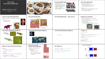
Texture Mapping May 4, 2006 Many slides are borrowed from UNC-CH - PDF document

Texture Mapping May 4, 2006 Many slides are borrowed from UNC-CH COMP236 Course (Spring 2003) taught by Leonard McMillan http://www.unc.edu/courses/2003spring/ comp/236/001/handouts.html 1

2

3

4

5

6

Compare the above with what we discussed previously… (Note the different meaning of s and t.) 7

Derivation of s and t • Two end points P 1 =(x 1 , y 1 , z 1 ) and P 2 =(x 2 , y 2 , z 2 ). Let P 3 =(1-t)P 1 +(t)P 2 • After projection, P 1 , P 2 , P 3 are projected to (x ’ 1 , y ’ 1 ), (x ’ 2 , y ’ 2 ), (x ’ 3 , y ’ 3 ) in screen coordinates. Let (x ’ 3 , y ’ 3 )=(1-s)(x ’ 1 , y ’ 1 ) + s(x ’ 2 , y ’ 2 ). • (x ’ 1 , y ’ 1 ), (x ’ 2 , y ’ 2 ), (x ’ 3 , y ’ 3 ) are obtained from P 1 , P 2 , P 3 by:  x ' w   x   x ' w   x  1 1 1 2 2 2         y ' w y y ' w y         1 1 = 1 2 2 = 2 M , M         z ' w z z ' w z 1 1 1 2 2 2         w 1 w 1         1 2  x ' w   x   x   x  3 3 3 1 2         y ' w y y y         3 3 = 3 = − 1 + 2 M M (( 1 t ) t )         z ' w z z z 3 3 3 1 2         w 1 1 1         3 8

Since  x   x ' w   x   x ' w  1 1 1 2 2 2         y y ' w y y ' w         1 = 1 1 2 = 2 2 M , M         z z ' w z z ' w 1 1 1 2 2 2         w w 1 1         1 2 We have:  x ' w   x   x  3 3 1 2       y ' w y y       3 3 = − 1 + ⋅ 2 ( 1 t ) M t M       z ' w z z 3 3 1 2       w 1 1       3     x ' w x ' w 1 1 2 2     y ' w y ' w     = − 1 1 + 2 2 ( 1 t ) t     z ' w z ' w 1 1 2 2     w w     1 2 When P 3 is projected to the screen, we get ( x ’ 3 , y ’ 3 ) by dividing by w , so: − + ⋅ − + ⋅ ( 1 t ) x ' w t x ' w ( 1 t ) y ' w t y ' w = ( x ' , y ' ) ( 1 1 2 2 , 1 1 2 2 ) 3 3 − + ⋅ − + ⋅ ( 1 t ) w t w ( 1 t ) w t w 1 2 1 2 But remember that (x ’ 3 , y ’ 3 )=(1-s)(x ’ 1 , y ’ 1 ) + s(x ’ 2 , y ’ 2 ) Looking at x coordinate, we have − + ⋅ ( 1 t ) x ' w t x ' w − + ⋅ = ( 1 s ) x s x 1 1 2 2 1 2 − + ⋅ ( 1 t ) w t w 1 2 9

We may rewrite s in terms of t, w 1 , w 2 , x ’ 1 , and x ’ 2 . In fact, ⋅ ⋅ t w t w = = s 2 2 − + ⋅ + − ( 1 t ) w t w w t ( w w ) 1 2 1 2 1 or conversely ⋅ ⋅ s w s w = = t 1 1 ⋅ + − − + s w ( 1 s ) w s ( w w ) w 1 2 1 2 2 Surprisingly, x ’ 1 and x ’ 2 disappear. Texture Mapping II 10

What You Will Learn Today? • Bump maps • Mipmapping for antialiased textures • Projective textures • Shadow maps • Environment maps The Limits of Geometric Modeling •Although graphics cards can render over 10 million polygons per second, that number is insufficient for many phenomena –Clouds –Grass –Terrain –Skin 11

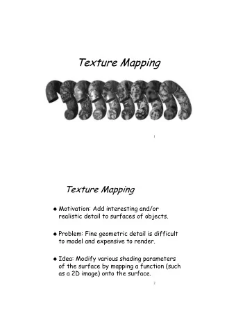
Modeling an Orange •Consider the problem of modeling an orange (the fruit) •Start with an orange-colored sphere –Too simple •Replace sphere with a more complex shape –Does not capture surface characteristics (small dimples) –Takes too many polygons to model all the dimples Modeling an Orange (2) •Take a picture of a real orange, scan it, and “paste” onto simple geometric model –This process is texture mapping •Still might not be sufficient because resulting surface will be smooth –Need to change local shape –Bump mapping 12

Three Types of Mapping •Texture Mapping –Uses images to fill inside of polygons •Environmental (reflection mapping) –Uses a picture of the environment for texture maps –Allows simulation of highly specular surfaces •Bump mapping –Emulates altering normal vectors during the rendering process Texture Mapping geometric model texture mapped 13

Environment Mapping Bump Mapping 14

Magnification and Minification More than one texel can cover a pixel ( minification ) or more than one pixel can cover a texel ( magnification ) Can use point sampling (nearest texel) or linear filtering ( 2 x 2 filter) to obtain texture values Texture Polygon Texture Polygon Magnification Minification Aliasing •Point sampling of the texture can lead to aliasing errors point samples in u,v (or x,y,z) space miss blue stripes point samples in texture space 15

Area Averaging A better but slower option is to use area averaging pixel preimage Note that preimage of pixel is curved 16

17

Example linear point filtering sampling mipmapped mipmapped point linear sampling filtering Automatic Texture Coordinate Generation • OpenGL can generate texture coordinates automatically glTexGen{ifd}[v]() • generation modes – GL_OBJECT_LINEAR – GL_EYE_LINEAR – GL_SPHERE_MAP (used for environmental maps) • Check the OpenGL Red Book! –4 th Ed., Chapter 8, pp.422-432, 446-450. 18

19

20

21

Shadow Map • Similarly, by clever use of glTexGen(), we can cast shadows on objects. With Shadows Without Shadows Figure 1. These diagrams were taken from Mark Kilgard’s shadow mapping presentation at GDC 2001. They illustrate the shadowing comparison that occurs in shadow mapping. More Detail • For projective texture, see: http://developer.nvidia.com/object/Proje ctive_Texture_Mapping.html • For shadow map, see: http://developer.nvidia.com/object/hwsh adowmap_paper.html 22

Question: Aren’t shadow and reflection global illumination effects? Why can we do it in the hardware pipeline? 23

24

25