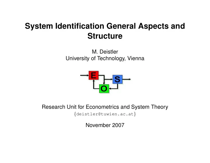
System Identification General Aspects and Structure M. Deistler - - PowerPoint PPT Presentation

System Identification General Aspects and Structure

• M. Deistler

University of Technology, Vienna Research Unit for Econometrics and System Theory

{deistler@tuwien.ac.at}

November 2007

1

Contents

• 1. Introduction
• 2. Structure Theory
• 3. Estimation for a Given Subclass
• 4. Model Selection
• 5. Linear Non-Mainstream Cases
• 6. Nonlinear Systems
• 7. Present State and Future Developments

November 2007

2

• 1. Introduction

The art of identification is to find a good model from noisy data: Data driven modeling. This is an important problem in many fields of application. Systematic approaches: Statistics, System Theory, Econometrics, Inverse Problems. MAIN STEPS IN IDENTIFICATION

• Specify the model class (i.e. the class of all a priori feasible candidate

systems): Incorporation of a priori knowledge.

• Specify class of observations.

November 2007

3

• Identification in the narrow sense. An identification procedure is a rule (in

the automatic case a function) attaching a system from the model class to the data ⋆ Development of procedures. ⋆ Evaluation of procedures (Statistical and numerical properties). Here only identification from equally spaced, discrete time data yt, t = 1, . . . T; yt ∈ Rs is considered. MAIN PARTS

• Main stream theory for linear systems (Nonlinear!).
• Alternative approaches to linear system identification.
• Identification of nonlinear systems: parametric, nonparametric

November 2007

4

MAINSTREAM THEORY

• The model class consists of linear, time-invariant, finite dimensional, causal

and stable systems only. The classification of the variables into inputs and

• utputs is given a priori.
• Stochastic models for noise are used; in particular noise is assumed to be

stationary, ergodic with a rational spectral density.

• The observed inputs are assumed to be free of noise and to be

uncorrelated with the noise process.

• Semi-nonparametric approach: A parametric subclass is determined by

model selection procedures. First step: Estimation of integer valued parameters. Then, for the given subclass, the finite dimensional vector of real valued parameters is estimated.

• Emphasis on asymptotic properties (consistency,

asymptotic distribution) in evaluation.

November 2007

5

3 MODULES IN IDENTIFICATION

• STRUCTURE THEORY: Idealized Problem;

we commence from the stochastic processes generating the data (or their population moments) rather than from data. Relation between “external behavior” and “internal parameters”.

• ESTIMATION OF REAL VALUED PARAMETERS: Subclass (dynamic

specification) is assumed to be given and parameter space is a subset of an Euclidean space and contains a nonvoid open set: M-estimators

• MODEL SELECTION: In general, the orders, the relevant inputs or even

the functional forms are not known a priori and have to be determined from

• data. In many cases, this corresponds to estimating a model subclass

within the original model class. This is done, e.g. by estimation of integers, e.g. using information criteria or test sequences.

November 2007

6

THE HISTORY OF THE SUBJECT (i) Early (systematic, methodological) time series analysis dates back to the 18th and 19th century. Main focus was the search for “hidden”periodicities and trends, e.g. in the orbits of planets (Laplace, Euler, Lagrange, Fourier). Periodogram (A. Schuster). Economic time series, e.g. for business cycle data. (ii) Yule (1921, 1923). Linear stochastic systems (MA and AR systems) used for explaining “almost periodic” cycles: yt − a1yt−1 − a2yt−2 = ǫt. (iii) (Linear) Theory of (weak sense) stationary processes (Cramer, Kolmogoroff, Wiener, Wold). Spectral representation, Wold representation (linear systems), factorization, prediction, filtering and interpolation.

November 2007

7

(iv) Early econometrics, in particular, the work of the Cowles Commission (Haavelmo, Koopmans, T. W. Anderson, Rubin, L. Klein). theory of identifiability and of (Gaussian) Maximum Likelihood (ML) - estimation for (finite dimensional) MIMO (multi-input, multi-output) linear systems (vector difference equations) with white noise errors (ARX systems). The maximum lag lengths are assumed to be known a priori. Development of LIML, 2SLS and 3 SLS estimators (T. W. Anderson, Theil, Zellner). (v) (Nonparametric) Spectral estimation and estimation of transfer functions (Tukey). (vi) Estimation of AR, ARMA, ARX and ARMAX systems. SISO (single-input,single-output) case. Emphasis on consistency, asymptotic normality and efficiency, in particular, for least squares and ML estimators. (T.W. Anderson, Hannan, Walker). (vii) Structure theory for (MIMO) state space and ARMA systems (Kalman).

November 2007

8

(viii) Box-Jenkins procedure: An “integrated” approach to SISO system identification including order estimation (non automatic), the treatment of certain non-stationarities and numerically efficient ML algorithms. Big impact on applications. (ix) Automatic procedures for order estimation, in particular, procedures based

• n information criteria (like AIC, BIC) (Akaike, Rissanen).

(x) Main stream theory for linear system identification (including MIMO systems): Structure theory, order estimation, estimation for “real valued” parameters with emphasis on asymptotic theory (Hannan, Akaike, Caines, Ljung). (xi) Alternative approaches.

November 2007

9

• 2. Structure Theory

Relation between external behavior and internal parameters. Linear, main stream case: Relations between transfer function and parameters. Main model classes for linear systems:

• AR(X)
• ARMA(X)
• State Space Models

Here, for simplicity of notation we assume that we have no observed inputs. In many applications AR models still dominate.

November 2007

10

Advantages of AR models:

• no problems of non-identifiability, structure theory is simple
• maximum likelihood estimates are of least squares type, i.e. asymptotically

efficient and easy to calculate Disadvantages of AR models:

• less flexible

November 2007

11

Here, the focus is on state space models. State space forms in innovation representation: xt+1 = Axt + Bεt (1) yt = Cxt + εt (2) where

• yt: s-dimensional outputs
• xt: n-dimensional states
• (εt) white noise
• A ∈ Rn×n, B ∈ Rn×s, C ∈ Rs×n: parameter matrices
• n: integer valued parameter

November 2007

12

Assumptions: |λmax(A)| < 1 (3) |λmax(A − BC)| ≤ 1 (4) Eεtε

′

t

= Σ > 0 (5) Transfer function: k(z) =

∞

• j=1

Kjzj + I Kj = CAj−1B (6)

November 2007

13

ARMA forms a(z)yt = b(z)εt External behavior f(λ) = (2π)−1k(e−iλ)Σk∗(e−iλ) f ↔ (k, Σ) Note that ARMA and state space systems describe the same class of transfer functions.

November 2007

14

Relation to internal parameters: (6) or a−1b = k UA = {k| rational, s × s, k(0) = I, no poles for |z| ≤ 1 and no zeros for |z| < 1} M(n) ⊂ UA: Set of all transfer functions of order n. TA: Set of all A, B, C for fixed s, but n variable, satisfying (4) and (5). S(n) ⊂ TA: Subset of all (A, B, C) for fixed n. Sm(n) ⊂ S(n): Subset of all minimal (A, B, C). π : TA → UA : π(A, B, C) = k = C(Iz−1 − A)−1B + I π is surjective but not injective

November 2007

15

Note: TA is not a good parameter space because:

• TA is infinite dimensional
• lack of identifiability
• lack of “well posedness”: There exists no continuous selection from the

equivalence classes π−1(k) for Tα.

November 2007

16

Desirable properties of parametrizations:

• UA and TA are broken into bits, Uα and Tα, α ∈ I, such that π restricted to

Tα: π|Tα : Tα → Uα is bijective. Tα is reparametrized such that it contains an

• pen set in an embeddding Rdα. By τ ∈ Tα we denote the vector of free
• parameters. Then there exists a parametrization ψα : Uα → Tα such that

ψα(π(A, B, C)) = (A, B, C) ∀(A, B, C) ∈ Tα.

• Uα is finite dimensional in the sense that Uα ⊂ ∪n

i=1M(i) for some n.

• Well posedness: The parametrization ψα : Uα → Tα is a homeomorphism

(pointwise topology Tpt for UA).

• Differentiability
• Uα is Tpt-open in ¯

Uα.

• ∪α∈IUα is a cover for UA.

November 2007

17

Examples:

• Canonical forms based on M(n), e.g. echelon forms and balanced
• realizations. Decomposition of M(n) into sets Uα of different dimension.

Nice free parameters vs. nice spaces of free parameters.

• “Overlapping description” of the manifold M(n) by local coordinates.
• “Full parametrization” for state space systems. Here S(n) ⊂ Rn2+2ns or

Sm(n) are used as parameter spaces for ¯ M(n) or M(n), respectively. Lack

• f identifiability. The equivalence classes are n2 dimensional manifolds.

The likelihood function is constant along these classes.

• Data driven local coordinates (DDLC): Orthonormal coordinates for the 2ns

dimensional ortho-complement of the tangent space to the equivalence class at an initial estimator. Extensions: slsDDLC and orthoDDLC

• ARMA systems with prescribed column degrees.

November 2007

18

• ARMA parametrizations commencing from writing k as c−1p where c is a

least common denominator polynomial for k and where the degrees of c and p serve as integer valued parameters. In general, state space systems have larger equivalence classes compared to ARMA systems: More freedom in selection of optimal representatives. Main unanswered question: Optimal tradeoff between “number” and dimension of the pieces Uα. Problem: Numerical properties of parametrizations Different parametrizations: ψ1 : U1 → T1 ⊂ TA ψ2 : U2 → T2 ⊂ TA

November 2007

19

STATISTICAL ANALYSIS (“real world”): For the asymptotic analysis, in the case that U1 ⊃ U2, U2 contains a nonvoid

• pen (in U1) set and k0 ∈ int U2, we have no essential differences in asympotic

theory:

• coordinate free consistency:
• different asymptotic distributions, but we know the transformation

NUMERICAL ANALYSIS (“integer world”):

• The selection from the equivalence class matters
• Dependence on algorithm

November 2007

20

Questions:

• What are appropriate evaluation criteria for numerical properties?
• Which are the optimal parameter spaces (algorithm specific)?

Relation between statistical and numerical precision: curvature of the criterion function:

November 2007

21

Consider the case s = n = 1 where (a, b, c) ∈ R3:

• Minimality: b = 0 and c = 0
• Equivalence classes of minimal systems: ¯

a = a, ¯ b = tb, ¯ c = ct−1, t ∈ R \ {0}

−2 2 −10 −5 5 10 −8 −6 −4 −2 2 4 6 8 B StabOber for γ=−1 DDLC for initial StabOber StabOber for γ=1 MinOber for γ=−1 Echelon A C −10 −5 5 10 −8 −6 −4 −2 2 4 6 8 B C

November 2007

22

• 3. Estimation for a Given Subclass

We here assume that Uα is given, we commence from data. Identifiable case: ψα : Uα → Tα has the desirable properties. τ ∈ Tα ⊂ Rdα: vector of free parameters for Uα. σ ∈ Σ ⊂ R

n(n+1) 2

: free parameters for Σ > 0. Overall parameter space: Θ = Tα × Σ. Many identification procedures, at least asymptotically, commence from the sample second moments of the data

November 2007

23

GENERAL FEATURES: ˆ γ(s) = T −1

T −s

• t=1

yt+sy

′

t,

s ≥ 0 Now, ˆ γ can be directly realized as an MA system typically of order Ts; ˆ ˆ kT IDENTIFICATION:

• Projection step (Model reduction). Important for statistical qualities.
• Realization step:

November 2007

24

Two types of procedures:

• Optimization based procedures, M-estimators:

ˆ θT = argminLT(θ; y1, . . . , yT)

• Direct procedures: Explicit functions. e. g. instrumental variables methods,

subspace methods.

November 2007

25

GAUSSIAN MAXIMUM LIKELIHOOD: ˆ LT(θ) = T −1log detΓT(θ) + T −1y′(T)ΓT(θ)−1y(T) where y(T) = (y′

1, . . . , y′ T)′, ΓT(θ) = Ey(T; θ)y

′(T; θ) and

ˆ θT = argminθ∈Θˆ LT(θ)

• No explicit formula for MLE, in general.
• ˆ

LT(k, Σ) since ˆ LT depends on τ only via k: parameter free approach.

• Boundary points are important.

WHITTLE LIKELIHOOD: ˆ LW,T(k, σ) = log detΣ + (2π)−1 π

−π

tr

• k(e−iλ)Σk∗(e−iλ)

−1 I(λ)

• dλ

where I(λ) is the periodogram.

November 2007

26

EVALUATION:

• Coordinate free consistency: for k0 ∈ Uα and

lim T −1 T −s

t=1 εt+sε

′

t = δ0,sΣ0 a.s. for s ≥ 0 we have ˆ

kT → k0 a.s. and ˆ ΣT → Σ0 a.s. Consistency proof: basic idea Wald (1949) for i.i.d. case. Noncompact parameter spaces: limT →∞ ˆ LT(k, σ) = L(k, σ) = log detΣ + (2π)−1 π

−π tr

• k(e−iλ)Σk∗(e−iλ)

−1 k0(e−iλ)Σ0k∗

0(e−iλ)

• dλ

a.s. (7) ⋆ L has a unique minimum at k0, Σ0. ⋆ (ˆ kT, ˆ ΣT) enters a compact set, uniform convergence in (7).

• Analogous for k0 ∈ ¯

Uα.

• Generalized, coordinate free consistency for k0 ∈ ¯

Uα, (ˆ kT, ˆ ΣT) → D a.s D: Set of all best approximants to k0, Σ0 in ¯ Uα × Σ.

November 2007

27

• Consistency in coordinates: ψα(ˆ

kT) = ˆ τT → τ0 = ψα(k0) a.s.

• CLT:

Under E(εt|Ft−1) = 0 and E(εtε′

t|Ft−1) = Σ0.

√ T(ˆ τT − τ0) →d N(0, V ) Idea of proof: Cramer (1946) i.i.d. case: Linearization.

November 2007

28

Direct Estimators: IV Methods, subspace methods: Numerically faster, in many cases not asymptotically efficient. CALCULATIONS OF ESTIMATES Usual procedure: consistent initial estimator (e.g. IV or subspace estimator) + one Gauss-Newton step gives an asymptotically efficient procedure (e.g. Hannan-Rissanen)

November 2007

29

HOWEVER THERE ARE STILL PROBLEMS

• Problem of local minima: “good” initial estimates are required
• Numerical problems: Optimization over a grid

Statistical accuracy may be higher than numerical accuracy Valleys close to equivalence classes corresponding to lower dimensional systems “Intelligent” parametrization may help DDLC’s and extensions: Data driven selection of coordinates from an uncountable number of possibilities Only locally homeomorphic

• “Curse of dimensionality”

lower dimensional parametrizations (e.g. reduced rank models) concentration of the likelihood function by a least squares step.

November 2007

30

• 4. Model Selection

Automatic vs. nonautomatic procedures. Information criteria: Formulate tradeoff between fit and complexity. Based on e.g. Bayesian arguments, coding theory . . . Order estimation (or more general closure nested case): n1 < n2 implies ¯ M(n1) ⊂ ¯ M(n2) and dim(M(n1)) <dim(M(n2)). Criteria of the form A(n) = log detˆ ΣT(n) + 2ns · c(T) · T −1 where ˆ ΣT(n) is the MLE for Σ0 over ¯ M(n) × Σ. c(T) = 2: AIC criterion c(T) = c·logT, c ≥ 1: BIC criterion

November 2007

31

Estimator: ˆ nT =argminA(n) Statistical evaluation: ˆ nT is consistent for lim

T →∞

c(T) T = 0, lim inf

T →∞

c(T) log log T > 0 Evaluation of uncertainty coming from model selection for estimators of real valued parameters. Note: Complexity is in the eye of the beholder. Consider e.g. AR models for s = 1: yt + a1yt−1 + a2yt−2 = εt Parameter spaces: T = {(a1, a2) ∈ R2|1 + a1z + a2z2 = 0 for |z| ≤ 1} T0 = {(0, 0)} T1 = {(a1, 0)||a1| < 1, a1 = 0} T2 = T − (T0 ∪ T1)

November 2007

32

Bayesian justification:

• Positive priors for all classes, otherwise MLE is asymptotically efficient.
• Certain properties of Uα, α ∈ I are needed, e.g. for BIC to give consistent

estimators: closure nestedness, e.g. n1 < n2 ⇒ ¯ M(n1) ⊂ ¯ M(n2) and dimM(n1) < dimM(n2). Main open question:

• Optimal tradeoff between dimension and “number” of pieces.

November 2007

33

Problem: Properties of post model selection estimators

• The statistical analysis of the MLE ˆ

τT traditionally does not take into account the additional uncertainty coming from model selection.

• This may result in very misleading conclusions

Consider AR case (nested): yt = a1yt−1 + . . . + apyt−p + εt where Tp =      a1 . . . ap   ∈ Rp|stability    The estimator (LS) for given p is ˆ τp = (X(p)′X(p))−1 X(p)y

November 2007

34

The post model selection estimator is ˜ τ =   . . .   1{ˆ

p=0} +

  ˆ a1(1) . . .   1{ˆ

p=1} + . . . +

  ˆ a1(p) . . . ˆ ap(p)   1{ˆ

p=p}

Main problem:

• Essential lack of uniformity in convergence of finite sample distributions.

November 2007

35

• 5. Linear Non-Mainstream Cases
• Time varying parameters
• Long memory
• Unstable systems, integration and cointegration
• Symmetric modeling, errors in variables, dynamic factor models,

identification in closed loop TIME VARYING PARAMETERS:

• Slowly varying parameters: Without and with models for time variation. e.g.

yt = atyt−1 + εt at = at−1 + vt Recursive, adaptive estimation. Estimating the speed of variation. November 2007

36

• Structural changes:

at = a(1) for t ≤ T0 a(2) for t > T0 Change point detection.

• STARX Models (Smooth Transition)

yt = a(1)yt−1 + d(1)zt + (a(2)yt−1 + d(2)zt)G(st; θ) + εt st . . . Transition variable G( . ; θ) : R − → [0, 1]

November 2007

37

LONG MEMORY: e.g. a simple fractionally integrated process of the form (1 − z)dyt = εt , s = 1, d ∈ (0.5, 0) yt = εt +

∞

• j=1

kjεt−j kj = (j!)−1d(d + 1) . . . (d + j − 1)

• j |kj| = ∞
• j k2

j < ∞

non-rational transfer function f(λ) ∼ λ−2d for λ − → 0

November 2007

38

COINTEGRATION: A stochastic process is called integrated (of order 1) if (1 − z)yt is stationary, while (yt) is not. An integrated vector process (yt) is called cointegrated if ∃α ∈ Rs such that (α′yt) is stationary. Motivation:

• Trends in means and variance
• α describes long run equilibrium

November 2007

39

STRUCTURE THEORY, AR CASE a(z)yt = εt SPECIAL REPRESENTATION (Johansen) (1 − z)yt = Γ1(1 − z)yt−1 + . . . + Γp−1(1 − z)yt−p+1 + Πyt−p + εt where Π = −a(1) and rk(Π) = s ⇔ (yt) is stationary rk(Π) = 0 ⇔ (yt) is integrated, but not cointegrated rk(Π) = r

• 0<r<s

⇔ (yt) is cointegrated with r l.i. c. v. Π = BA′, A, B ∈ Rs×r. The rows of A span the cointegrating space. November 2007

40

MLE, AR CASE

• (Gaussian) likelihood ˜

LT(Γ1, . . . , Γp−1, Σ, B, A)

• Concentrated likelihood (stepwise) ˆ

LT(A, r): likelihood ratio tests ⋆ H0: at most r (r < s) l.i. cointegrating vectors ⋆ H1: r + 1 l.i. cointegrating vectors

• Nonstandard limiting distributions for the test under H0
• Asymptotic properties for the MLE’s ˆ

AT and ˆ BT under additional normalization: non-normal limiting distributions, different speeds of convergence.

November 2007

41

Simplest case: AR(1), scalar yt = ρyt−1 + εt OLS estimate ˆ ρT: √ T(ˆ ρT − ρ) →d N(0, 1 − ρ2) for |ρ| < 1 T(ˆ ρT − 1) →d

1 2(W(1)2 − 1)

1

0 W(r)2dr

for ρ = 1 where W(.) is the standard Brownian motion; functional CLT’s and continuous mapping theorem.

• LR tests and MLE’s are available
• Open problems in structure theory and specification

November 2007

42

LINEAR DYNAMIC FACTOR MODELS: Basic model yt = Λ(z)ξt + ut , Eξtu

′

s = 0

yt: s-dimensional observations ξt: r < s-dimensional factors, in general unobserved Λ(z) =

i Λjzj:

factor loadings ˆ y = Λ(z)ξt: latent variables Spectral densities fy(λ) = Λ(e−ıλ)fξ(λ)Λ∗(e−ıλ) + fu(λ) Idea: Dimension reduction in cross section and time, modeling high dimensional time series, using information contained in additional time series.

November 2007

43

Tasks:

• Estimation of (low dimensionally parametrized versions of)

Λ(z), fξ(λ), fu(λ)

• Estimation of factor processes (ξt)
• Forecasting

Problems:

• Identifibiality
• Estimation of real valued parameters
• Model selection, in paricular determinig r from data.
• Estimation of factors

November 2007

44

Additional a-priori information has to be imposed, otherwise the problem would be ”completely non identifiable”. Special model classes:

• (Dynamic) principal compenents

fy(λ) = O1(λ)fξ(λ)O∗

1(λ) + O2(λ)Ω2(λ)O∗ 2(λ)

where O1, O2 : eigenvectors offy

• fξ

Ω2

• :

eigenvalues offy ξt = O∗

1(z)yt

, ut = O2O∗

2yt

November 2007

45

Interpretation: Best (Frobenius norm) approximation of fy(λ) by rank r matrices, or best approximation of observations (yt) by latent variables ( ˆ yt).

• Dynamic factor model with idiosyncratic noise

Assumption: fu is diagonal Basic idea: Separation of common and of individual components: Splitting property: The factors make the component-processes of (yt) conditionally uncorrelated. Identifiability problems: Ledermann bound In general the factors are no functions of the observations. MLE; tests for the number of factors

• Generalized dynamic factor model: fu is not necessarily diagonal, but the
• ff-diagonal elements are ”small”. Identifiability only for s → ∞ (and r

const.). Approximation by PCA.

November 2007

46

• 6. Nonlinear Systems

Nonlinear system identification is a word like “non-elephant zoology”

• Asymptotic theory for M-estimation in parametric classes of nonlinear

(dynamic) systems. Party analogous to the case of linear models; no general structure theory available.

• Nonparametric estimation for nonlinear time series models, e.g. by kernel
• methods. Nonlinear autoregressions yt = g(yt−1, . . . , yt−p) + εt. Asymptotic

theory, rates of convergence.

• Semi-nonparametric estimation, e.g. by dynamic neural nets. “Universal

approximation properties” (nonlinear black box models).

• Special classes of nonlinear systems, e.g. GARCH type models.
• Chaos models: nonlinearity instead of stochasticity.

November 2007

47

ARCH and GARCH models Modeling of volatility clustering: ARCH: εt = σtzt σ2

t

= c +

p

• i=1

αiε2

t−i

where zt is IID with Ezt = 0 and Ez2

t = 1, c > 0, αi ≥ 0.

Stationarity condition: p

i=1 αi < 1.

Note that (εt) is white noise but E(ε2

t|εt−1, εt−2, . . .) = c + α1ε2 t−1 + . . . + αpε2 t−p

November 2007

48

GARCH: εt = σtzt σ2

t

= c +

p

• i=1

αiε2

t−i + p

• i=1

βiσ2

t−i

where, in addition, β(z) = 1 − p

i=1 βizi = 0 for |z| ≤ 1 and βi ≥ 0.

Stationarity condition: (α1 + β1) + . . . (αp + βp) < 1 Used for forecasting risk

November 2007

49

• Estimation: MLE (ARCH case)

ˆ LT(c, αi, βi) = 1 T

• t

log(c +

• i

αiε2

t−i) + 1

T

• t

ε2

t

(c +

i αiε2 t−i)

The MLE’s are obtained by numerical optimization.

• Tests for conditional heteroskedasticity.

Testing for correlation in ε2

t.

Lagrange multiplier test (ARCH case: H0: α1 = . . . = αp = 0) Great number of extensions.

November 2007

50

• 7. Present State and Future Developments

PRESENT STATE:

• Theory and methods have reached a certain state of maturity. Large body
• f methods and theories available.

Demand pull rather than theory push. Increasing fragmentation corresponding to different fields of application (data structure, model classes, prior knowledge).

November 2007

51

• Boom in applications: Number of applications and areas of application are

increasing. Data compression & coding Signal extraction Analysis Forecasting Simulation Monitoring Control Estimation of “physically” meaningful parameters Empirical discrimination between conflicting theories                                                                           Signal processing Process modeling & control in engineering Finance Business & Marketing System biology Monitoring in medicine . . . “Component manufacturing” Enabling technology, not very visible

November 2007

52

• Different communities and multicultural:

Econometrics Statistics Systems & Control Signal processing Intruders, e.g. neural nets Shifting boundaries IMPORTANT PROBLEMS FOR THE FUTURE

• There are still major open problems in linear systems identification
• Highly structured systems, e.g. compartment models. Additional prior

information such as mass-balancing.

• Nonlinear systems
• Spatio-temporal systems, PDE’s
• Large data sets, high dimensional time series

November 2007

53

• Improved model selection and regularization procedures
• Further automatization
• Hybrid procedures
• Use of symbolic computation

CHANCES AND DANGERS The increasing number of applications poses challenges. Will there be still a common body of theory and methods? Danger of fragmentation and of becoming selfreferential.

November 2007