Synchronous Balanced Analysis Andreea Beica, Vincent Danos cole - PowerPoint PPT Presentation
Synchronous Balanced Analysis Andreea Beica, Vincent Danos cole Normale Suprieure Paris GT Bioss, 13 March 2017 1 Overview What? Piecewise synchronous approximation of Chemical Reaction Networks (CRN) dynamics Why? highlight
Synchronous Balanced Analysis Andreea Beica, Vincent Danos École Normale Supérieure Paris GT Bioss, 13 March 2017 1
Overview What? Piecewise synchronous approximation of Chemical Reaction Networks’ (CRN) dynamics Why? • highlight interdependence of cellular processes • finite cellular resource allocation VS cellular processes (i.e., growth) • rephrase mass action run of CRNs as an optimisation problem How? Resource allocation centred Petri Nets with maximal-step execution semantics Usage? Approximation of real dynamics, constraint-based model similar to Flux Balance Analysis Work in progress! 2
Motivation Cellular processes rarely work in isolation: the rest of the cell cannot be ignored. Finite cellular resources: committing to one task reduces the amount available to others Define a formal notion of “growth”: use as an improved biomass function in FBA Andrea Y. Weiße, Diego A. Oyarzún, Vincent Danos, and Peter S. Swain Mechanistic links between cellular trade-offs, gene expression, and growth PNAS 2015 112 (9) E1038-E1047; 2015, doi:10.1073/pnas.1416533112 3
Modeling CRNs CRN = <S, ∇ + , ∇ - , R, κ > PN = <P , T, W , m 0 > species reactions places initial marking { S 1 , . . . , S s } { R 1 , . . . , R r } m 0 : P → N stoichiometry matrices transitions r + 2 R r × s 8 s, t : r − ( s, t ) = W ( s, t ) r − 2 R r × s 8 s, t : r + ( s, t ) = W ( t, s ) r = r + � r − reaction rate constants κ : R → R > 0 W : (( S × T ) ∪ ( T × S )) → N 4
CRN mass action dynamics s s reaction: k i X X r + r i : ij S j ij S j r − � ! j =1 j =1 reaction network: k ! r + S r − S � system state: x = ( x S 1 , ..., x S s ) ∈ N s dx dt = ( r + � r � ) T · K · x r − CRN dynamics: K = diag ( κ 1 , ..., κ r ) vector-matrix exponentiation 5
Petri Nets & Chemical Reaction Networks κ 0 3 A + 2 B → A − κ 1 5 B + 3 C → 2 A + 2 B − κ 2 C → 2 B − m 0 = (9 , 9 , 9) 1 0 0 3 2 0 r + = r − = 2 2 0 0 5 3 0 2 0 0 0 1 6
Piecewise synchronous execution Split: Burst: Collect: 7
"SPLIT": resource allocation reaction Resource allocation matrix: α ij species α ∈ R | T | × | S | X ∀ j ∈ S, α ij ≤ 1 i ∈ T Interpretation: resource fraction VS reaction probability 8
"BURST": Max-parallel execution semantics of PN “ execute greedily as many transitions as possible in one step” Definition: A max-parallel execution step in a PN at state m is a positive T-vector v s.t.: 1. v is compatible with m: 0 m � r − v 2. v is exhaustive: 8 j 2 T, m � r − v ⇤ r j , where r j is the j th column of r − 9
"BURST": Max-parallel execution semantics of PN { t 0 × 3 , t 2 × 9 } { t 0 × 2 , t 1 , t 2 × 6 } 10
Resource allocation & Max Parallel Execution i ∈ S ( ↵ ji Define ( ↵ ? m ) j = min · m i ) r − ij Theorem: ∀ v compatible with a resource array m (and potentially max-parallel), ∃ ↵ resource allocation matrix s.t. v = ↵ ? m. Furthermore, if the CRN is unary, there is unicity of ↵ Our execution semantics encompasses max-parallel execution 11
Growth in unary CRNs State of the system after 1 execution with given α split: ( I + r · α ) · m State of the system after k executions with given α split: D k α · m, with D α = I + r · α X m = m i , with m i ∈ E ( λ i ) λ 1 > λ 2 > · · · , the eigenvalues of D α i ( λ i X D k α · m = λ k ) k · m i ] 1 · [ m 1 + λ 1 i ≥ 2 The growth rate of the system is given by λ 1. 12
Unary CRNs and Depletion Time S i → . . . @ k j ; j ∈ N i , | N i | = n S i → . . . @ k · log( α ji · S i (0) τ = k − 1 log( S i (0) τ j = k − 1 ) ) j s i,j s i depletion level 13
Unary CRNs: “iso” assumptions Decouple production and consumption Isochronous : ∀ j ∈ N i , τ j = τ Iso-remainder: ∀ j ∈ N i , s i,j = s i ∆ m ( ⌧ ) = r · ( ↵ i � ✏ i ) · m ∆ m ⇡ τ → 0 r · [ k j ] · m τ The usual ODE dynamics is recreated: dx dt = ( r + � r � ) T · K · x r − 14
Unary CRNs: “iso” assumptions e τ · k j − 1 ↵ S i ( ⌧ , ˆ ⇥ ⇤ ⇥ ⇤ ˆ k S i ) = = ↵ i − ✏ i P j 1 + e τ · k j Resource allocation matrix as a function of depletion time and reaction rate constants! 15
Concrete interpretation Approximation of system dynamics: τ α τ → 0 α ( τ , ˆ dx ˆ k ) dt = r T · K · x r − ∆ m ( ⌧ ) = r · ( ↵ i � ✏ i ) · m ˆ ✏ κ temporised discrete execution • “ don’t wait for the slowest reaction” • simulation: big step approx. of an integrator (deterministic tau-leaping) • 16
Abstract interpretation Synchronous Balanced Analysis Objective function: λ 1 ( λ i X D k α · m = λ k ) k · m i ] 1 · [ m 1 + λ 1 i ≥ 2 maximize α max α ( τ , ˆ ˆ k ) Constrain reaction rates, refute models 17
SBA VS.FBA able to handle growth (no steady state assumption needed) • take into account real system kinetics • characterise behaviour of a cell using only one construction: α • replace mechanistic details of resource allocation with an abstract vector • objective biomass function emerges directly from method: growth rate • maximising biggest eigenvalue of matrix: how ? •
Future work • binary reactions : depletion time? (Michaelis-Menten type assumption) • explore correlations between growth rate and model parameters • tau-leaping, whole-cell models by Karr, etc… 19
Conclusion Piecewise synchronous approximation of the dynamics of (growth) CRNs: parallel execution semantics of PN, based on resource allocation . Interpretations: 1. approx. of real system dynamics 2. constraint based method (like FBA) 20
Thank you!
Recommend
More recommend
Explore More Topics
Stay informed with curated content and fresh updates.
